Segmentation#
Separating an image into one or more regions of interest.#
Everyone has heard or seen Photoshop or a similar graphics editor take a person from one image and place them into another. The first step of doing this is identifying where that person is in the source image. This is an example of breaking the image into segments, where one segment represents the human, and other segments are not.
To take another example, self-driving cars use cameras, and therefore digital images, to look for (segment) important objects in their environment, such as other cars. Here’s an example where an image segmentation algorithm has split the input image (in the left panel) into segments (in the right panel), including a nearby car.

(Images from the Roboflow image segmentation dataset, licensed under CC-by-4.0).
There are various ways to segment images, many of them implemented in Scikit-image.
Segmentation contains two major sub-fields#
Supervised segmentation: Some prior knowledge, possibly from human input, is used to guide the algorithm. Supervised algorithms currently included in Scikit-image include:
Thresholding algorithms that require user input (
skimage.filters.threshold_*)skimage.segmentation.random_walker(starts with specified markers);skimage.segmentation.active_contour(“snake” starting coordinates);skimage.segmentation.watershed(basin starting coordinates);
Unsupervised segmentation: No prior knowledge. These algorithms attempt to subdivide into meaningful regions automatically. The user may be able to tweak settings like number of regions.
Thresholding algorithms which do not require user input.
skimage.segmentation.slicskimage.segmentation.chan_veseskimage.segmentation.felzenszwalbskimage.segmentation.quickshift
First, some standard imports and a helper function to display our results
import numpy as np

import matplotlib.pyplot as plt

import skimage as ski

# We will often use the segmentation sub-module in this page.
import skimage.segmentation as seg


def image_show(image, nrows=1, ncols=1, cmap='gray', **kwargs):
    """ Display intensity image with `plt.imshow`
    """
    fig, ax = plt.subplots(nrows=nrows, ncols=ncols, figsize=(16, 16))
    ax.imshow(image, cmap=cmap)
    ax.axis('off')
    return fig, ax
Thresholding#
In some images, global or local contrast may be sufficient to separate regions of interest. Simply choosing all pixels above or below a certain threshold may be sufficient to segment such an image.
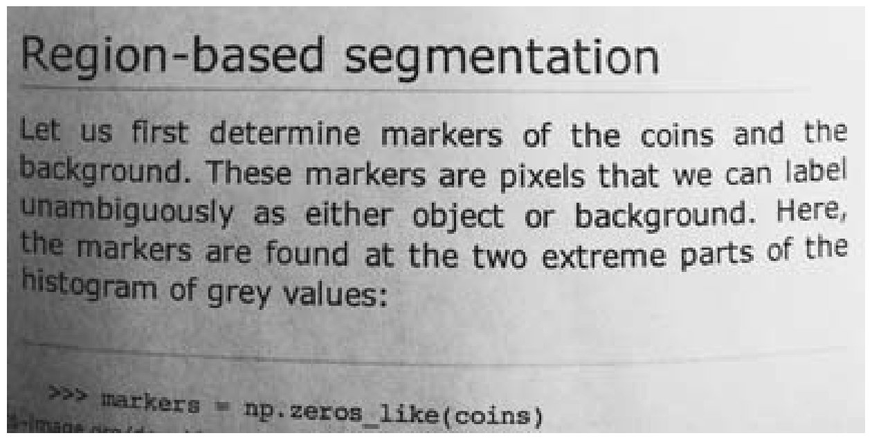
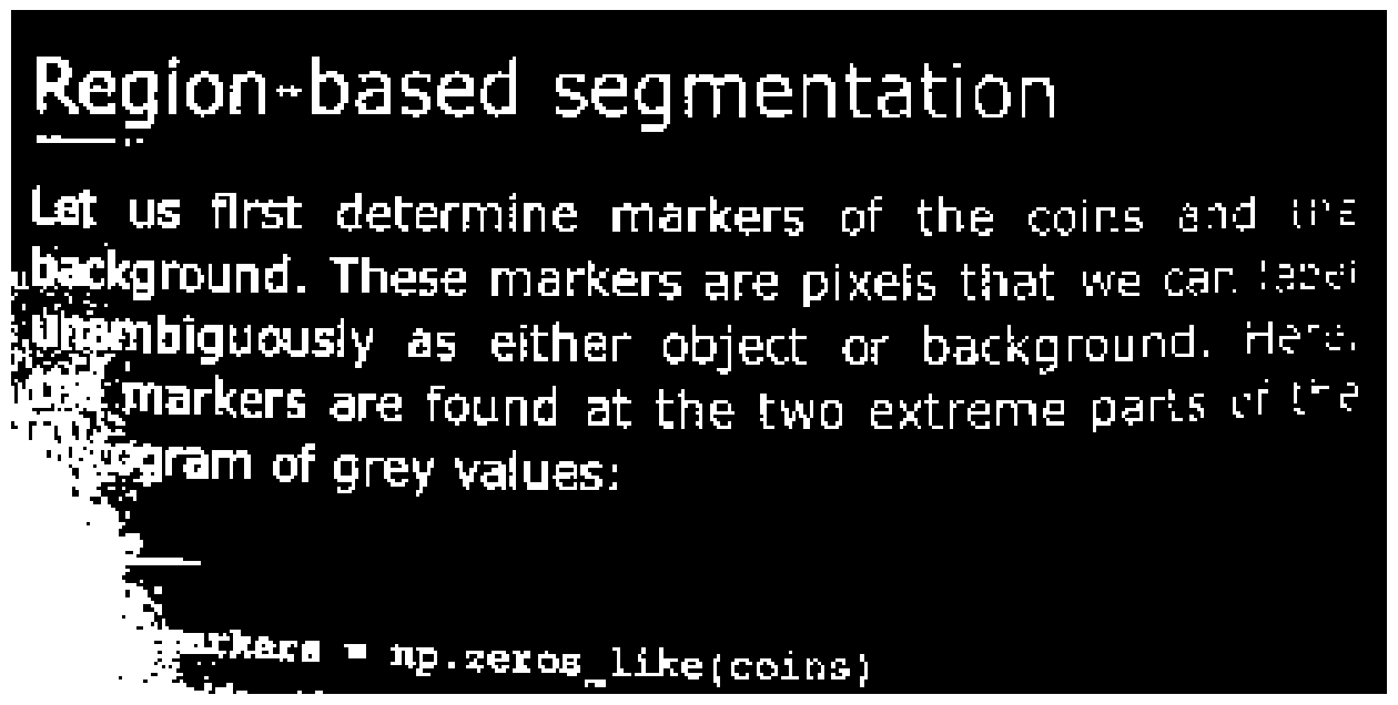
Let’s try this on an image of a textbook.
text = ski.data.page()
image_show(text);
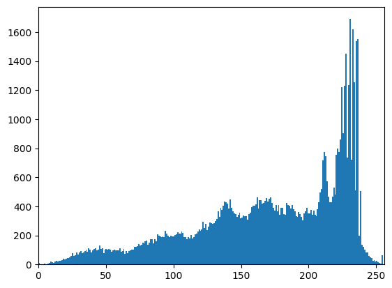
Histograms#
A histogram simply plots the frequency (number of times) values within a certain range appear against the data values themselves. It is a powerful tool to get to know your data - or decide where you would like to threshold.
fig, ax = plt.subplots(1, 1)
ax.hist(text.ravel(), bins=256, range=[0, 255])
ax.set_xlim(0, 256);
Experimentation: supervised thresholding#
Try simple NumPy methods and a few different thresholds on this image. Because we are setting the threshold, this is supervised segmentation.
text_segmented = text < 100  # Try different values here
image_show(text_segmented);
Not ideal results! The shadow on the left creates problems; no single global value really fits.
What if we don’t want to set the threshold every time? There are several published methods which look at the histogram and choose what should be an optimal threshold without user input. These are unsupervised.
Experimentation: unsupervised thresholding#
Here we will experiment with a number of automatic thresholding methods available in Scikit-image. Because these require no input beyond the image itself, this is unsupervised segmentation.
These functions generally return the threshold value(s), rather than applying it to the image directly.
Try otsu and li, then take a look at local or sauvola.
# Hit tab with the cursor after the underscore, try several methods
text_threshold = ski.filters.threshold_

image_show(text < text_threshold);
Supervised segmentation#
Thresholding can be useful, but is rather basic and a high-contrast image will often limit its utility. For doing more fun things - like removing part of an image - we need more advanced tools.
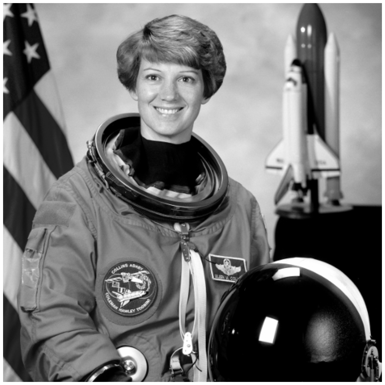
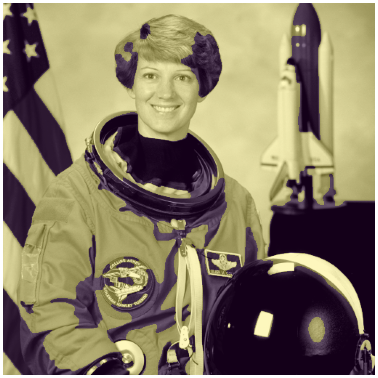
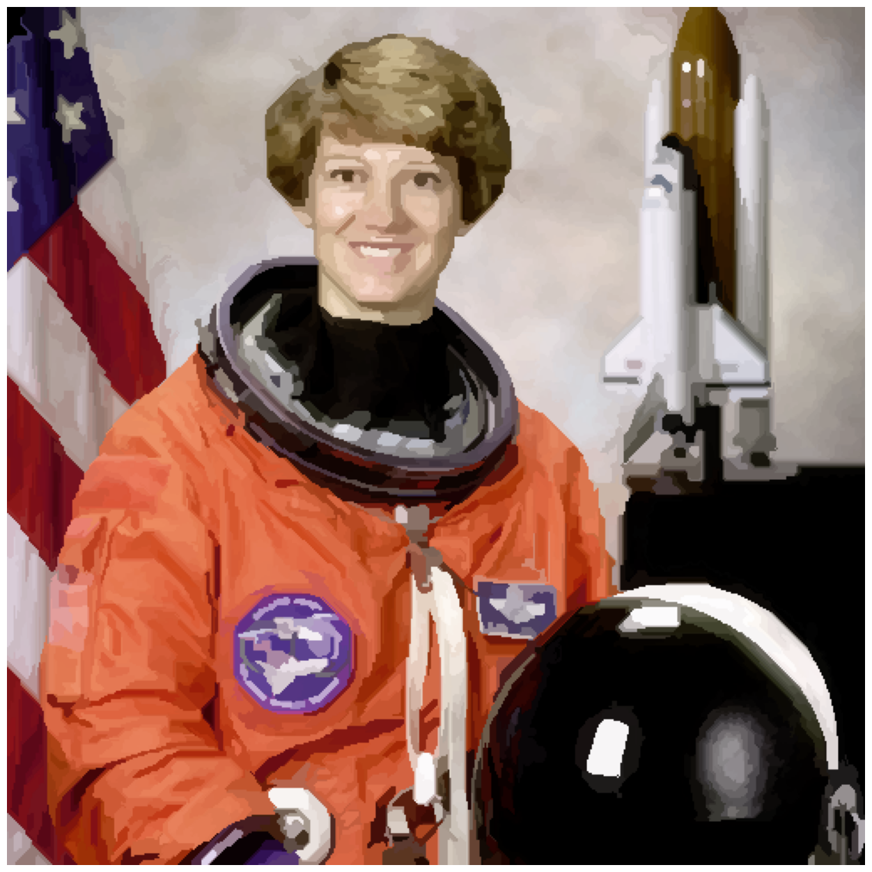
For this section, we will use the astronaut image and attempt to segment Eileen Collins’ head using supervised segmentation.
# Our source image
astronaut = ski.data.astronaut()
image_show(astronaut);

The contrast is pretty good in this image for her head against the background, so we will simply convert to grayscale with rgb2gray.
astronaut_gray = ski.color.rgb2gray(astronaut)
image_show(astronaut_gray);
We will use two methods, which segment using very different approaches:
Active Contour: Initializes using a user-defined contour or line, which then is attracted to edges and/or brightness. Can be tweaked for many situations, but mixed contrast may be problematic.
Random walker: Initialized using any labeled points, fills the image with the label that seems least distant from the origin point (on a path weighted by pixel differences). Tends to respect edges or step-offs, and is surprisingly robust to noise. Only one parameter to tweak.
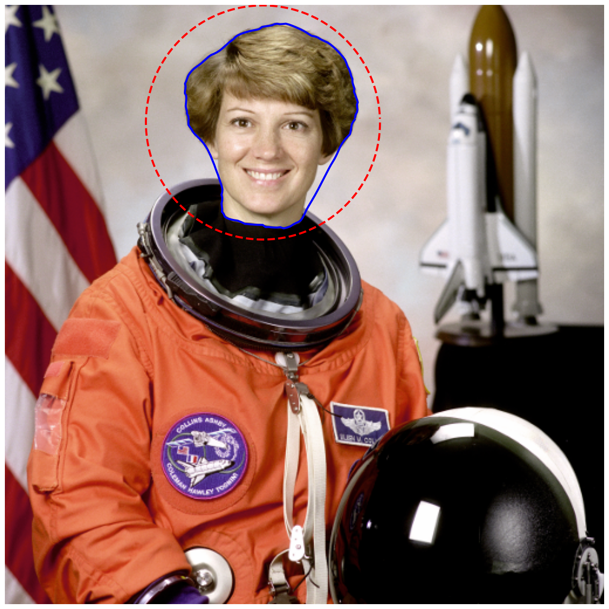
Active contour segmentation#
We must have a set of initial parameters to ‘seed’ our segmentation for this. Let’s draw a circle around the astronaut’s head to initialize the snake.
This could be done interactively, with a GUI, but for simplicity we will start at the point [100, 220] and use a radius of 100 pixels. We add just a little trigonometry in this helper function…
def circle_points(resolution, center, radius):
    """Generate points defining a circle on an image."""
    radians = np.linspace(0, 2*np.pi, resolution)

    r = center[0] + radius*np.sin(radians)
    c = center[1] + radius*np.cos(radians)

    return np.array([r, c]).T

# Exclude last point because a closed path should not have duplicate points
points = circle_points(resolution=200, center=[100, 220], radius=100)[:-1]
# Try different values for alpha.  Can you do better than we did?
snake = seg.active_contour(astronaut_gray, points, alpha=0.2)
fig, ax = image_show(astronaut)
ax.plot(points[:, 1], points[:, 0], '--r', lw=3)
ax.plot(snake[:, 1], snake[:, 0], '-b', lw=3);
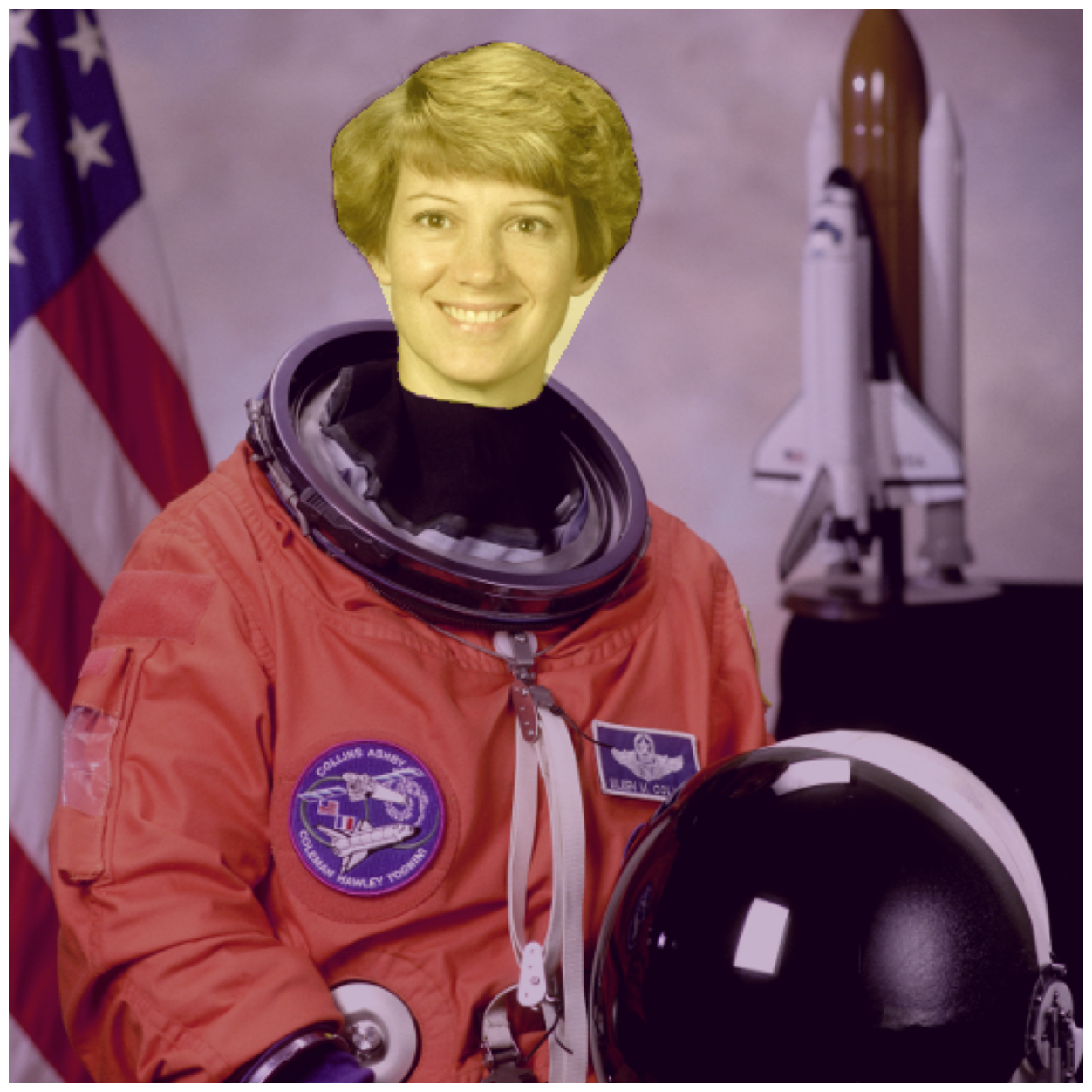
Aside — making masks from contours#
snake above contains a contour — that is, a line enclosing an area of
interest.
Sometimes we want to make a mask or region label from such a contour.
The trick to doing this, is to think of the contour as the vertices (points) defining a polygon in Scikit-image terms.
A polygon is a shape defined by points (vertices).
ski.draw.polygon returns row and column indices for all points inside the
polygon.
Here is ski.draw.polygon in action, for the snake contour above:
mask_shape = astronaut.shape[:-1]  # 2D mask shape (no color).
face_mask = np.zeros(mask_shape)
in_face_rows, in_face_cols = ski.draw.polygon(snake[:, 0],
                                              snake[:, 1],
                                              mask_shape)
face_mask[in_face_rows, in_face_cols] = 1
fig, ax = image_show(astronaut)
ax.imshow(face_mask, alpha=0.3);
Random walker#
One good analogy for random walker uses graph theory.
The distance from each pixel to its neighbors is weighted by how similar their values are; the more similar, the lower the cost is to step from one to another
The user provides some seed points
The algorithm finds the cheapest paths from each point to each seed value.
Pixels are labeled with the cheapest/lowest path.
We will reuse the seed values from our previous example.
astronaut_labels = np.zeros(astronaut_gray.shape, dtype=np.uint8)
The random walker algorithm expects a label image as input. Any label above zero will be treated as a seed; all zero-valued locations will be filled with labels from the positive integers available.
There is also a masking feature where anything labeled -1 will never be labeled or traversed, but we will not use it here.
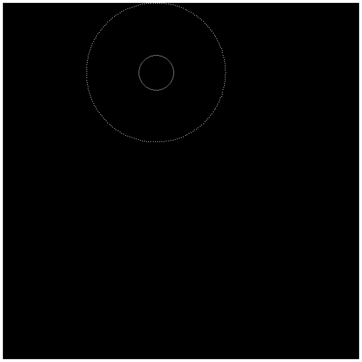
indices = ski.draw.circle_perimeter(100, 220, 25)

astronaut_labels[indices] = 1
astronaut_labels[points[:, 0].astype(int), points[:, 1].astype(int)] = 2

image_show(astronaut_labels);
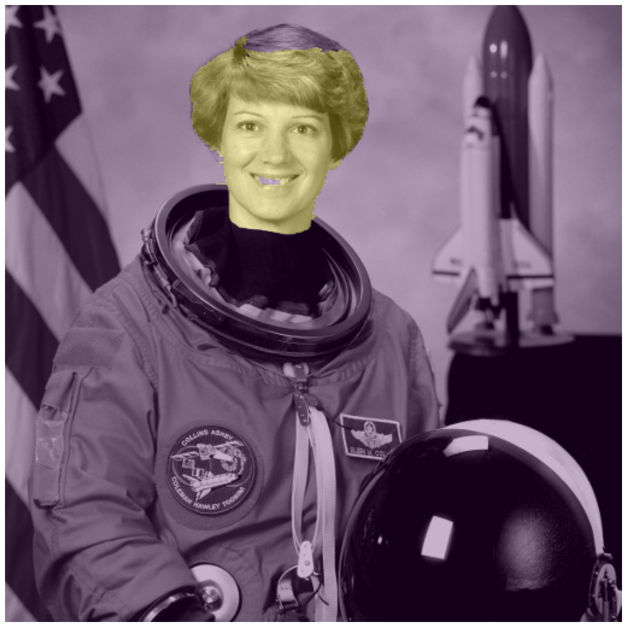
# Experiment with different beta values here.  Can you do a better job than we have?
astronaut_segmented = seg.random_walker(astronaut_gray, astronaut_labels, beta=2500)
/opt/hostedtoolcache/Python/3.13.11/x64/lib/python3.13/site-packages/skimage/_shared/utils.py:587: UserWarning: The probability range is outside [0, 1] given the tolerance `prob_tol`. Consider decreasing `beta` and/or decreasing `tol`.
  return func(*args, **kwargs)
# Check our results
fig, ax = image_show(astronaut_gray)
ax.imshow(astronaut_segmented == 1, alpha=0.3);
Flood fill#
segmentation.flood and segmentation.flood_fill are basic but effective
segmentation techniques. These algorithms take a seed point and iteratively
find and fill adjacent points which are equal to or within a tolerance of the
initial point. flood returns the region; flood_fill returns a modified
image with those points changed to a new value.
This approach is most suited for areas which have a relatively uniform color or gray value, and/or high contrast relative to adjacent structures.
Can we accomplish the same task with flood fill?
seed_point = (100, 220)  # Experiment with the seed point
flood_mask = seg.flood(astronaut_gray, seed_point, tolerance=0.3)  # Experiment with tolerance
fig, ax = image_show(astronaut_gray)
ax.imshow(flood_mask, alpha=0.3)
ax.plot(220, 100, 'bo');  # Show the seed point.
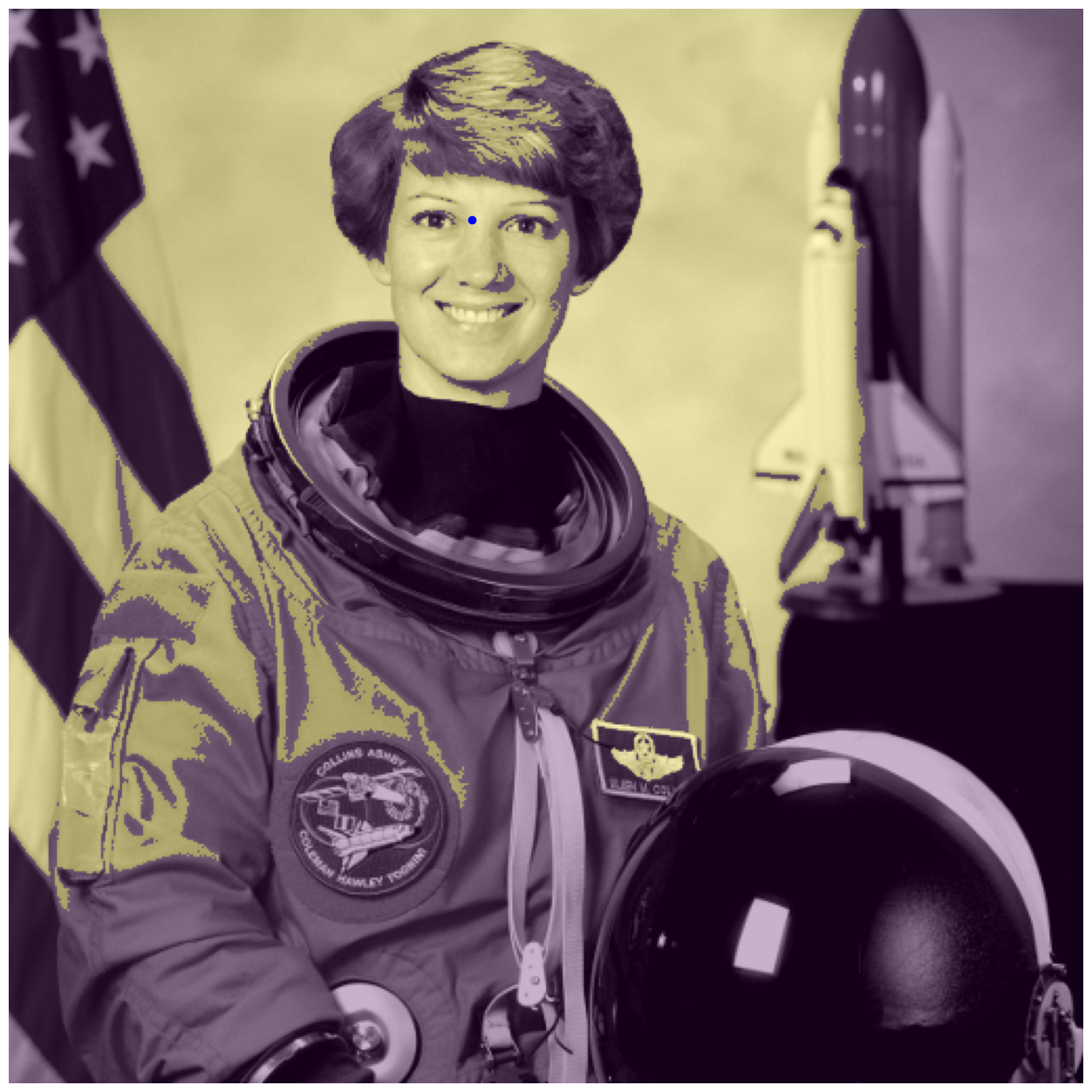
With our initial tolerance=0.3, the results are not ideal! The flood runs away into the background through the right earlobe.
Let’s think outside the box:
What if instead of segmenting the head, we segmented the background around it and the collar?
Is there any way to increase the contrast between the background and skin?
seed_bkgnd = (100, 350)  # Background
seed_collar = (200, 220)  # Collar

better_contrast = ...  # Your idea to improve contrast here
tol_bkgnd = ...   # Experiment with tolerance for background
tol_collar = ...  # Experiment with tolerance for the collar

flood_background = seg.flood(better_contrast, seed_bkgnd, tolerance=tol_bkgnd)
flood_collar = seg.flood(better_contrast, seed_collar, tolerance=tol_collar)
fig, ax = image_show(better_contrast)

# Combine the two floods with binary OR operator
ax.imshow(flood_background | flood_collar, alpha=0.3);
flood_mask2 = seg.flood(astronaut[..., 2], (200, 220), tolerance=40)
fig, ax = image_show(astronaut[..., 2])
ax.imshow(flood_mask | flood_mask2, alpha=0.3);
Unsupervised segmentation#
Sometimes, human input is not possible or feasible - or, perhaps your images are so large that it is not feasible to consider all pixels simultaneously. Unsupervised segmentation can then break the image down into several sub-regions, so instead of millions of pixels you have tens to hundreds of regions.
SLIC#
There are many analogies to machine learning in unsupervised segmentation. Our first example directly uses a common machine learning algorithm under the hood - K-Means.
# SLIC works in color, so we will use the original astronaut
astronaut_slic = seg.slic(astronaut)
# label2rgb replaces each discrete label with the average interior color
image_show(ski.color.label2rgb(astronaut_slic, astronaut, kind='avg'));
We’ve reduced this image from 512*512 = 262,000 pixels down to 100 regions!
And most of these regions make some logical sense.
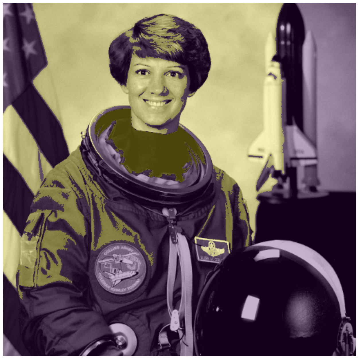
Chan-Vese#
This algorithm iterates a level set, which allows it to capture complex and even disconnected features. However, its result is binary - there will only be one region - and it requires a grayscale image.
This algorithm takes a few seconds to run.
chan_vese = seg.chan_vese(astronaut_gray)
fig, ax = image_show(astronaut_gray)
ax.imshow(chan_vese == 0, alpha=0.3);
Chan-Vese has a number of parameters, which you can try out! In the interest of time, we may move on.
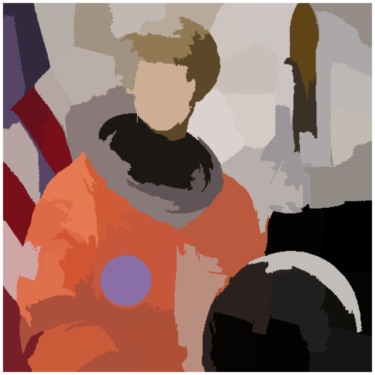
Felzenszwalb#
This method oversegments an RGB image (requires color, unlike Chan-Vese) using another machine learning technique, a minimum-spanning tree clustering. The number of segments is not guaranteed and can only be indirectly controlled via scale parameter.
astronaut_felzenszwalb = seg.felzenszwalb(astronaut) # Color required
image_show(astronaut_felzenszwalb);

Exercise 28
We found lots of regions! How many is that?
# Find the number of unique labels
n_labels = ...
To see if the labels make sense, label them with the region average (see above with SLIC):
astronaut_felzenszwalb_colored = ... # Your code here

image_show(astronaut_felzenszwalb_colored);
Solution to Exercise 28
n_labels = np.unique(astronaut_felzenszwalb).size
n_labels
3295
To label the regions with the region average:
astronaut_felzenszwalb_colored = ski.color.label2rgb(
    astronaut_felzenszwalb,
    astronaut,
    kind='avg')
image_show(astronaut_felzenszwalb_colored);
If you did the exercise, you will know that we have a large number of
reasonably small regions. If we wanted fewer regions, we could change the
scale parameter (try it!) or start here and combine them.
This approach is sometimes called oversegmentation.
But when there are too many regions, they must be combined somehow.
Combining regions with a Region Adjacency Graph (RAG)#
Remember how the concept behind random walker was functionally looking at the difference between each pixel and its neighbors, then figuring out which were most alike? A RAG is essentially the same, except between regions.
We have RAGs in Scikit-image, in the graph sub-module:
rag = ski.graph.rag_mean_color(astronaut, astronaut_felzenszwalb + 1)
Now we show just one application of a very useful tool - skimage.measure.regionprops - to determine the centroid of each labeled region and pass that to the graph.
regionprops has many, many other uses; see the regionprops API
documentation
for all of the features that can be quantified per-region!
# Regionprops ignores zero, but we want to include it, so add one
regions = ski.measure.regionprops(astronaut_felzenszwalb + 1)

# Pass centroid data into the graph
for region in regions:
    rag.nodes[region['label']]['centroid'] = region['centroid']
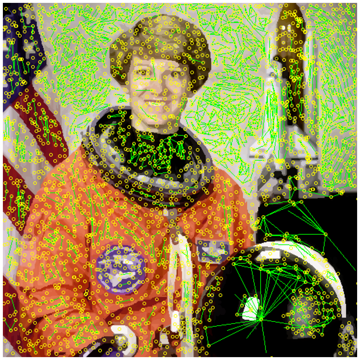
display_edges is a helper function to assist in visualizing the graph.
def display_edges(image, g, threshold):
    """Draw edges of a RAG on its image
    Returns a modified image with the edges drawn.Edges are drawn in green
    and nodes are drawn in yellow.

    Parameters
    ----------
    image : ndarray
        The image to be drawn on.
    g : RAG
        The Region Adjacency Graph.
    threshold : float
        Only edges in `g` below `threshold` are drawn.

    Returns:
    out: ndarray
        Image with the edges drawn.
    """
    image = image.copy()
    for edge in g.edges():
        n1, n2 = edge

        r1, c1 = map(int, rag.nodes[n1]['centroid'])
        r2, c2 = map(int, rag.nodes[n2]['centroid'])

        line  = ski.draw.line(r1, c1, r2, c2)
        circle = ski.draw.circle_perimeter(r1,c1, 2)
        if g[n1][n2]['weight'] < threshold :
            image[line] = 0,255,0
        image[circle] = 255,255,0

    return image
# All edges are drawn with threshold at infinity
edges_drawn_all = display_edges(astronaut_felzenszwalb_colored, rag, np.inf)
image_show(edges_drawn_all);
Try a range of thresholds out, see what happens.
threshold = 5 # Experiment with this value.  You can do better than this.

edges_drawn_few = display_edges(astronaut_felzenszwalb_colored, rag, threshold)
image_show(edges_drawn_few);
Finally, cut the graph#
Once you are happy with the (dis)connected regions above, the graph can be cut to merge the regions which are still connected.
final_labels = ski.graph.cut_threshold(astronaut_felzenszwalb + 1, rag, threshold)
final_label_rgb = ski.color.label2rgb(final_labels, astronaut, kind='avg')

image_show(final_label_rgb);

How many regions exist now?
np.unique(final_labels).size
1813
Exercise 29
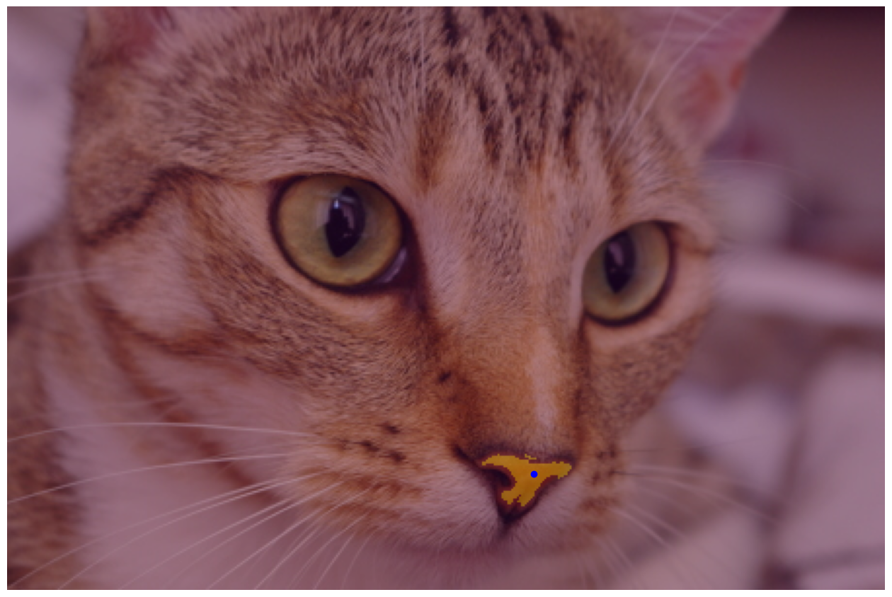
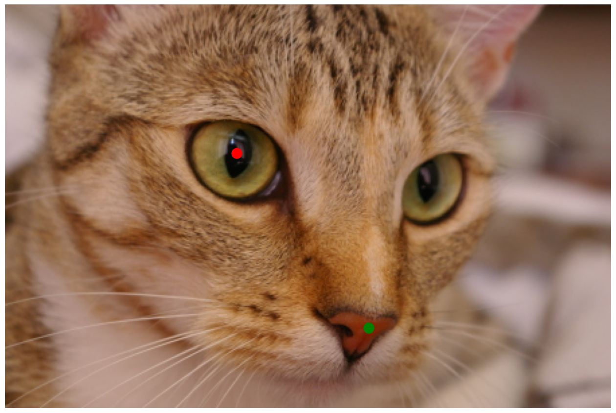
The data directory also has an excellent image of Stéfan’s cat, Chelsea. With what you’ve learned, can you segment the cat’s nose? How about the right eye? Why is the eye particularly challenging?
Specifically, please define mask images for each region. That is, define
a 2D image reye_mask that has 0 for pixels outside Chelsea’s right eye, and
1 for pixels inside. Similarly, define nose_mask with 0 for pixels outside
Chelsea’s nose, and 1 for pixels inside the nose area.
We’ve given you starting coordinates for Chelsea’s nose and right eye, but you can choose your own if you prefer.
chelsea = ski.data.chelsea()
fig, ax = image_show(chelsea)

nose = np.array([270, 240])
reye = np.array([172, 110])

ax.plot(nose[0], nose[1], marker='o', markersize=15, color="g")
ax.plot(reye[0], reye[1], marker='o', markersize=15, color="r");
Hint : the nose is a strangely difficult problem. You might consider trying filtered versions of the image to first detect the edges defining the nose (and other edges), and then find the pixels inside the nose area from the filtered image. But any successful method is fine.
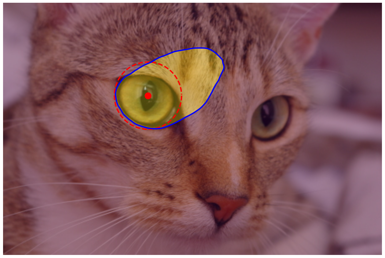
Solution to Exercise 29
cat_gray = ski.color.rgb2gray(chelsea)

# Use the utility routine above.
reye_points = circle_points(resolution=200, center=reye[::-1], radius=40)[:-1]
# Refine the circle with an active contour to get the outline.
reye_snake = seg.active_contour(cat_gray, points, alpha=0.23)

# Make a region from the outline.
reye_mask = np.zeros(cat_gray.shape)
rows, cols = ski.draw.polygon(reye_snake[:, 0],
                              reye_snake[:, 1],
                              cat_gray.shape)
reye_mask[rows, cols] = 1

# Show the circle, refined contour and region
fig, ax = image_show(chelsea)
ax.imshow(reye_mask, alpha=0.3)

ax.plot(reye[0], reye[1], marker='o', markersize=15, color="r");
ax.plot(reye_points[:, 1], reye_points[:, 0], '--r', lw=3)
ax.plot(reye_snake[:, 1], reye_snake[:, 0], '-b', lw=3);
cat_sobel = ski.filters.sobel(chelsea[..., 0])
nose_mask = seg.flood(cat_sobel, tuple(nose)[::-1], tolerance=0.03)

fig, ax = image_show(chelsea)
ax.imshow(nose_mask, alpha=0.3)
ax.plot(*nose, 'bo');  # Show the seed point.