Threshold filtering#
Note
This tutorial is adapted from “Image manipulation and processing using NumPy and SciPy” by Emmanuelle Gouillart and Gaël Varoquaux, and “scikit-image: image processing” by Emmanuelle Gouillart. Please see the References section at the end of the page for other sources and resources.
A common operation we will want to perform on images is filtering. This is where we modify the pixels in an image according to a certain rule or algorithm, often based on a specific pixel intensity value, or the pixel intensity values of other pixels within the “local neighborhood” of a given pixel. Filtering techniques can be used to remove noise from an image, or to achieve specific visual effects, amongst other purposes.
Here we will look at threshold filtering where we filter an image based on
specific pixel intensity values. We will show how threshold filtering works at
the pixel-level, using numpy and scipy, and then we will show how to apply
it in skimage.
# Library imports.
import numpy as np
import matplotlib.pyplot as plt
import scipy.ndimage as ndi
import skimage as ski

# Set 'gray' as the default colormap
plt.rcParams['image.cmap'] = 'gray'

# Set NumPy precision to 2 decimal places
np.set_printoptions(precision=2)

# Custom functions for illustrations, and to quickly report image
# attributes.
from skitut.noise_illustration import generate_image, original_image
from skitut import show_attributes
What is signal? What is noise?#
Imagine that I want to send you a picture message. Let’s use “the signal” as the name for the image before I send it to you. Before transmission, the signal (image) has a clear meaning which I am confident you will be able to interpret. However, imagine that I am sending you the message via an unreliable medium; a messaging system that is prone to corrupting messages when transmitting them.
When I send you the message, there is a decent chance that unwanted randomness will be added to the image file, because of technical problems with the transmission medium. This might result in an image which contains so much randomness that it is hard to discern the original signal.
Imagine that the cell below attempts to send my picture message - can you see what the signal is?
# Generate a noisy image array.
# generate_image is our own function to generate the image and add noise.
noisy = generate_image()
show_attributes(noisy)
plt.imshow(noisy);
Type: <class 'numpy.ndarray'>
dtype: float64
Shape: (7, 7)
Max Pixel Value: 1.0
Min Pixel Value: -0.95
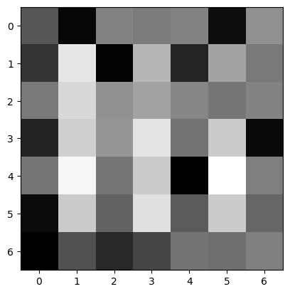
Any ideas? Maybe you can determine what signal is in there, but we trust that it is at least somewhat ambiguous, to most readers.
We saw simple threshold filtering on an earlier
page. This is where we select
a threshold value, and binarize the image using that value. So a given pixel
becomes True if a pixel is more intense than the threshold, and False if
it is lower (or vice versa, depending on the comparison operator).
The aim here is typically to split the pixels into distinct classes, based on their intensity values. We can use the ndarray .ravel() method to view a histogram of the pixel intensities, in order to find a threshold that might be useful to use in a filter. The .ravel() method “flattens” the image array to 1-D, so that it can be displayed as a histogram:
# The `shape` of the original `noisy` image.
print(noisy)
noisy.shape
[[-0.29 -0.9   0.05 -0.01  0.06 -0.84  0.15]
 [-0.55  0.8  -0.93  0.44 -0.67  0.3  -0.02]
 [-0.02  0.7   0.16  0.3   0.08 -0.05  0.05]
 [-0.68  0.63  0.2   0.78 -0.07  0.6  -0.88]
 [-0.05  0.93 -0.05  0.6  -0.95  1.    0.02]
 [-0.86  0.59 -0.19  0.75 -0.25  0.6  -0.17]
 [-0.94 -0.33 -0.64 -0.42 -0.06 -0.1   0.03]]
(7, 7)
# Flatten to 1-D with the `.ravel()` method.
print(noisy.ravel())
noisy.ravel().shape
[-0.29 -0.9   0.05 -0.01  0.06 -0.84  0.15 -0.55  0.8  -0.93  0.44 -0.67
  0.3  -0.02 -0.02  0.7   0.16  0.3   0.08 -0.05  0.05 -0.68  0.63  0.2
  0.78 -0.07  0.6  -0.88 -0.05  0.93 -0.05  0.6  -0.95  1.    0.02 -0.86
  0.59 -0.19  0.75 -0.25  0.6  -0.17 -0.94 -0.33 -0.64 -0.42 -0.06 -0.1
  0.03]
(49,)
When we plot a histogram of the flattened image array, what we are doing is dividing the \(x\)-axis into intervals (e.g. 0 to 0.25), and then getting a count of how many pixel intensity values fall within each \(x\)-axis interval:
# Show a histogram of the pixel intensity values, from the "flattened" `noisy` array.
plt.hist(noisy.ravel(),
         bins=13) # Set a reasonable number of x-axis intervals.
plt.xlabel('Pixel Intensity Value')
plt.ylabel('Pixel Count');
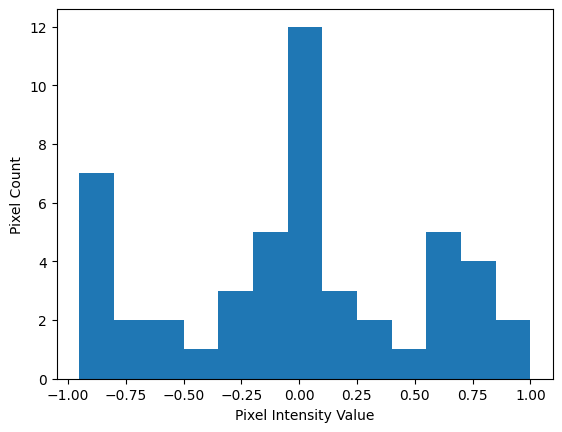
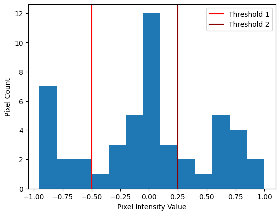
Ok, so it looks like the distribution is trimodal. The message image is in the float64 dtype, using intensities ranging from -1 to 1. Let’s set a threshold filter for each dip, in between the three peaks. So, we’ll try once with a threshold of -0.50, and once with a threshold of 0.25. These threshold values are shown as vertical lines on the plot below:
# Show a histogram of the pixel intensity values, with some thresholds.
plt.hist(noisy.ravel(), bins=13)
plt.axvline(-0.5, color='red', label='Threshold 1')
plt.axvline(0.25, color='darkred', label='Threshold 2')
plt.legend()
plt.xlabel('Pixel Intensity Value')
plt.ylabel('Pixel Count');
The filters are applied into binary images, using the > comparison operator,
in the next two cells:
# The first simple, Boolean threshold filter.
simple_threshold_filter_1 = noisy > -0.50
simple_threshold_filter_1
array([[ True, False,  True,  True,  True, False,  True],
       [False,  True, False,  True, False,  True,  True],
       [ True,  True,  True,  True,  True,  True,  True],
       [False,  True,  True,  True,  True,  True, False],
       [ True,  True,  True,  True, False,  True,  True],
       [False,  True,  True,  True,  True,  True,  True],
       [False,  True, False,  True,  True,  True,  True]])
# The second simple, Boolean threshold filter.
simple_threshold_filter_2 = noisy > 0.25
simple_threshold_filter_2
array([[False, False, False, False, False, False, False],
       [False,  True, False,  True, False,  True, False],
       [False,  True, False,  True, False, False, False],
       [False,  True, False,  True, False,  True, False],
       [False,  True, False,  True, False,  True, False],
       [False,  True, False,  True, False,  True, False],
       [False, False, False, False, False, False, False]])
Each threshold filter is just a Boolean array, with the same .shape as the image. When we render these arrays with Matplotlib, we will see a binary image, where True values are mapped to white and False values are mapped to 0.
Because we used the > comparison operator, only pixels larger than the threshold values will be True. Let’s see if this clears up any of the noise:
# Threshold filters.
plt.figure(figsize=(10, 4))
plt.subplot(1, 2, 1)
plt.title('Threshold = -0.5')
plt.imshow(simple_threshold_filter_1)
plt.subplot(1, 2, 2)
plt.title('Threshold = 0.25')
plt.imshow(simple_threshold_filter_2);
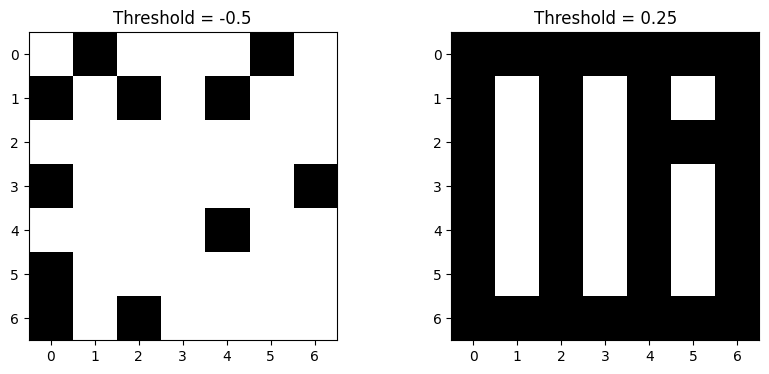
Ok, so the first image still looks very noisy still, but the second looks like we might be getting somewhere. Maybe you can already guess what the original signal was…
Let’s loop through some other threshold values, between just below 0 to just larger than 0.25, to see if the clarity of the signal improves:
# Loop through some different threshold values, and plot the results.
plt.figure(figsize=(16, 8))
n_plots=6
for i, val in enumerate(np.linspace(start=-0.1,
                                    stop=0.25,
                                    num=n_plots)):
    plt.subplot(2, int(n_plots/2), i+1)
    plt.title(f"Threshold =\n {val.round(2)}")
    plt.imshow(noisy > val)
    plt.axis('off')
plt.tight_layout();
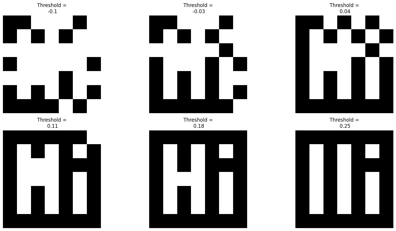
We hope you feel suitably greeted! The threshold of 0.18 seems to reveal the original signal in this image, before the unwanted random noise was added, by the faulty transmission system.
Here we have recovered a signal from a noisy image, and made the features in the image easier to discern. You’ll notice that we had to try numerous threshold values to find the “sweet spot” with the best results. Other values “overshoot” and “undershoot” the optimum value.
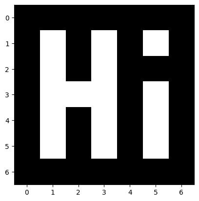
Here was the original image, before the noise was added:
plt.imshow(original_image());
Reducing noise and enhancing image features are both common aims in image filtering. Both processes often require some trial and error with different values for optional arguments that go into the filtering operation, as it did here. We will now turn to some other common methods for threshold filtering, using a variety of other images.
Threshold filtering is just Boolean filtering#
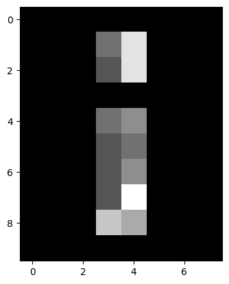
As we have seen, threshold filtering involves modifying pixel values based on a threshold value. Let’s investigate other thresholding methods using a grayscale image:
# Create a grayscale image array.
random_i = np.array([[0, 0, 0, 0, 0, 0, 0, 0],
                     [0, 0, 0, 4, 8, 0, 0, 0],
                     [0, 0, 0, 3, 8, 0, 0, 0],
                     [0, 0, 0, 0, 0, 0, 0, 0],
                     [0, 0, 0, 4, 5, 0, 0, 0],
                     [0, 0, 0, 3, 4, 0, 0, 0],
                     [0, 0, 0, 3, 5, 0, 0, 0],
                     [0, 0, 0, 3, 9, 0, 0, 0],
                     [0, 0, 0, 7, 6, 0, 0, 0],
                     [0, 0, 0, 0, 0, 0, 0, 0]])
random_i
array([[0, 0, 0, 0, 0, 0, 0, 0],
       [0, 0, 0, 4, 8, 0, 0, 0],
       [0, 0, 0, 3, 8, 0, 0, 0],
       [0, 0, 0, 0, 0, 0, 0, 0],
       [0, 0, 0, 4, 5, 0, 0, 0],
       [0, 0, 0, 3, 4, 0, 0, 0],
       [0, 0, 0, 3, 5, 0, 0, 0],
       [0, 0, 0, 3, 9, 0, 0, 0],
       [0, 0, 0, 7, 6, 0, 0, 0],
       [0, 0, 0, 0, 0, 0, 0, 0]])
plt.imshow(random_i);
As we saw above, it is simple to create a Boolean mask filter, using the >
comparison operator:
# Create a Boolean array using a comparison operator.
random_i_thresholded = random_i > 5
print(random_i_thresholded)
plt.matshow(random_i_thresholded);
[[False False False False False False False False]
 [False False False False  True False False False]
 [False False False False  True False False False]
 [False False False False False False False False]
 [False False False False False False False False]
 [False False False False False False False False]
 [False False False False False False False False]
 [False False False False  True False False False]
 [False False False  True  True False False False]
 [False False False False False False False False]]
This filters out pixels below the threshold value (5), by setting them to 0/False. Different threshold values will allow more or less pixels to “survive” the filtering operation:
# A sole survivor!
random_i_filtered_9 = random_i >= 9
print(random_i_filtered_9)
plt.matshow(random_i_filtered_9);
[[False False False False False False False False]
 [False False False False False False False False]
 [False False False False False False False False]
 [False False False False False False False False]
 [False False False False False False False False]
 [False False False False False False False False]
 [False False False False False False False False]
 [False False False False  True False False False]
 [False False False False False False False False]
 [False False False False False False False False]]
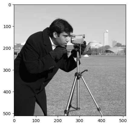
Image segmentation via threshold filtering#
This threshold filtering technique can be useful for segregating the
foreground from the background of real images, like camera:
# Get the `camera` image from `ski.data`.
camera = ski.data.camera()
# Show the "raw" `camera` array.
camera
array([[200, 200, 200, ..., 189, 190, 190],
       [200, 199, 199, ..., 190, 190, 190],
       [199, 199, 199, ..., 190, 190, 190],
       ...,
       [ 25,  25,  27, ..., 139, 122, 147],
       [ 25,  25,  26, ..., 158, 141, 168],
       [ 25,  25,  27, ..., 151, 152, 149]], shape=(512, 512), dtype=uint8)
# Show `camera` graphically.
plt.imshow(camera);
We can again use the NumPy .ravel() method of the camera array to allow us to view a histogram of the pixel intensities. We set the number of bins (\(x\)-axis intervals) for the histogram to be 128, to keep the plot looking smooth:
# Plot a histogram of the `camera` pixel intensities, with 128 bins.
histogram = plt.hist(camera.ravel(), bins=128)
plt.xlabel('Pixel Intensity Value')
plt.ylabel('Pixel Count');

The “bins” are the intervals along the \(x\)-axis in which pixel intensity values are counted to determine the height of the blue “hills” in the histogram above, within a given interval. It is important, when thresholding, to choose a sensible number of bins. With too few bins, we miss important information, because we are cramming many disparate pixel intensity values into one bin. Too many bins and we clutter our histogram with lots of spikes which occlude the general pattern.
To illustrate this, the plot below shows the camera pixel intensity histograms, with too few and too many bins. The bin interval starts and ends are indicated with vertical red lines. The height on the histogram, for a given bin, is determined by the Pixel Count falling with the range of intensities for that bin:
# Some plot formatting parameters (to show the bins).
marker = '|'
color = 'red'
markersize = 40

# Too few bins...
plt.figure(figsize=(16, 4))
n_bins_few = 4
plt.subplot(1, 2, 1)
histogram = plt.hist(camera.ravel(), bins=n_bins_few)
plt.title(f"{n_bins_few} bins. Too few!")
plt.xlabel('Pixel Intensity Value')
plt.ylabel('Pixel Count')
colors=['red', 'yellow']
for val in histogram[1]:
    plt.plot(val, 0, marker=marker,
             color = "red", markersize=markersize,
            markeredgewidth=8)

# Too many bins...
n_bins_many = 200
plt.subplot(1, 2, 2)
plt.title(f"{n_bins_many} bins. Too many!")
histogram = plt.hist(camera.ravel(), bins=n_bins_many)
plt.xlabel('Pixel Intensity Value')
plt.ylabel('Pixel Count')
for val in histogram[1]:
    plt.plot(val, 0, marker=marker, color = "red", markersize=markersize);
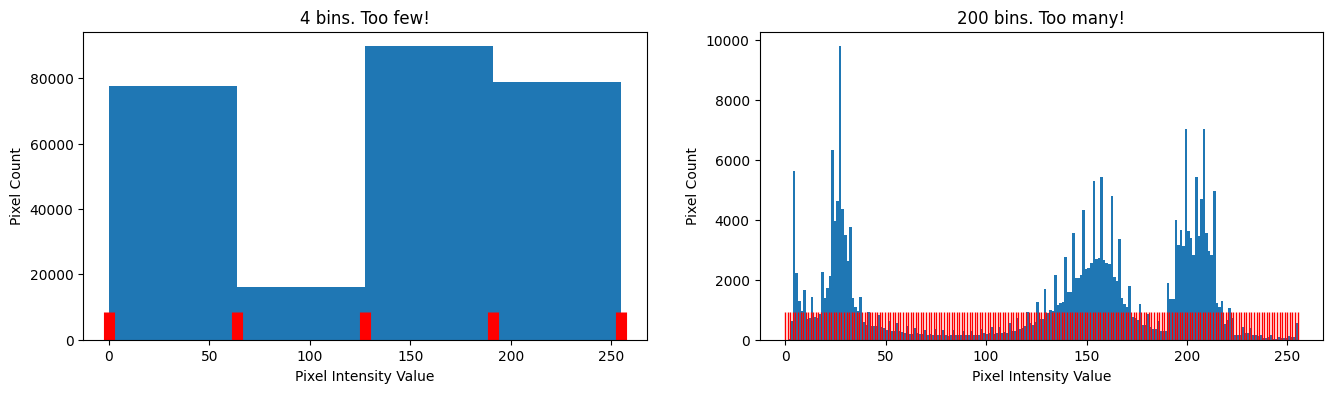
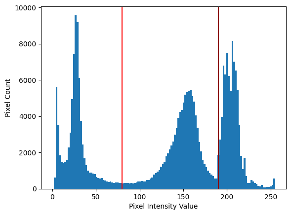
128 bins gives us a good middle ground, where we can see patterns in the distribution easily, without losing information or overemphasising unrepresentative values. Using the sensible number of bins, the distribution is clearly trimodal, with a clear dip/separation around around 50-100, and another just before 200. These locations are indicated on the plot with vertical lines:
# Show some "by eye" thresholds.
plt.hist(camera.ravel(), bins=128)
plt.axvline(80, color='red')
plt.axvline(190, color='darkred')
plt.xlabel('Pixel Intensity Value')
plt.ylabel('Pixel Count');
Let’s use these “by eye” crude threshold values and apply a threshold filter using them. Remember, our aim here is to separate the pixels into distinct classes; we hope these two distinct pixel classes will correspond to the foreground and background of the image:
# Define a threshold, "by eye".
crude_threshold = 80
# Apply the filter.
camera_threshold_filtered = camera.copy()
camera_threshold_filtered = camera_threshold_filtered < crude_threshold
plt.imshow(camera_threshold_filtered);
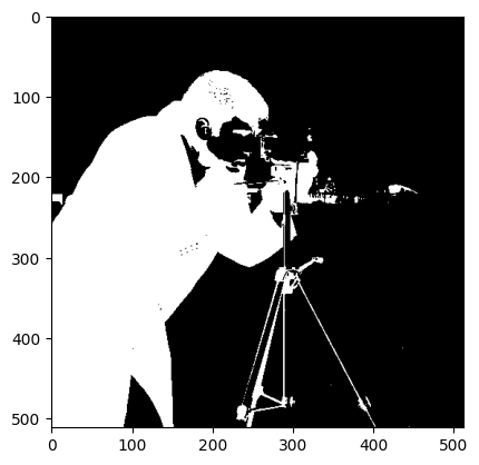
That has worked fairly well, as far as it goes, for segmenting the foreground (the cameraman) away from the background (the field and buildings behind the cameraman).
We can show the “opposite” binary image, by reversing the comparison operation:
# Using the "opposite" comparison operator.
plt.imshow(camera > crude_threshold);
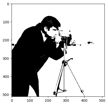
Stylish! Someone should put that on a t-shirt…
Threshold filters in skimage - the Otsu method#
skimage contains many threshold filters, the cell below uses the dir() function to show the available selection:
# Show the `skimage` threshold filters.
[fil for fil in dir(ski.filters) if fil.startswith('threshold')]
['threshold_isodata',
 'threshold_li',
 'threshold_local',
 'threshold_mean',
 'threshold_minimum',
 'threshold_multiotsu',
 'threshold_niblack',
 'threshold_otsu',
 'threshold_sauvola',
 'threshold_triangle',
 'threshold_yen']
These filters typically, when passed an image array, find threshold values
automatically - e.g. threshold values at which to divide the pixels into
distinct classes. These distinct pixel classes often correspond to distinct
features or regions in the image (cameraman vs field, foreground vs
background etc.). The threshold value searches performed by the
ski.filter.threshold* functions aim to maximize the separation between pixel
classes, and the different available functions use different algorithms to
identify the “best” threshold value(s).
One simple method, similar to the “look at the histogram” method we just used
above, is the Otsu method.
This aims to divide pixels into two distinct classes, by mathematically
analyzing a histogram of the pixel intensities. Below we use the
ski.filters.threshold_otsu() function to recommend a threshold value, at which to segment our image into two separate pixel classes.
By specifying the nbins argument, we instruct the .threshold_otsu() function to analyse a histogram which has the same number of bins as the one we were using above:
# Pass our `camera` array to the `threshold_otsu()` function.
otsu_thresh = ski.filters.threshold_otsu(camera, nbins=128)

# Show the Otsu threshold
otsu_thresh
np.int64(102)
We show the Otsu threshold (otsu_thesh) as a vertical line on the histogram below:
# Plot the pixel intensities, and the Otsu threshold.
plt.hist(camera.ravel(), bins=128);
plt.axvline(otsu_thresh, color='red', label='Otsu Threshold')
plt.xlabel('Pixel Intensity Value')
plt.ylabel('Pixel Count')
plt.legend();

You can see that the method finds a threshold is pretty close to the one we chose “by eye” earlier on the page. Let’s apply the Otsu filter, simply by using camera < otsu_thresh:
# Filter in the image using the Otsu threshold.
camera_otsu_filtered = camera < otsu_thresh

# Show a plot of the whole Otsu filtering process.
plt.figure(figsize=(14, 3))
plt.subplot(1, 3, 1)
plt.imshow(camera)
plt.title('Original')
plt.subplot(1, 3, 2)
plt.hist(camera.ravel(), bins=128)
plt.xlabel('Pixel Intensity Value')
plt.ylabel('Pixel Count')
plt.axvline(otsu_thresh, color='red')
plt.title('Otsu threshold')
plt.subplot(1, 3, 3)
plt.imshow(camera_otsu_filtered)
plt.title('Otsu filtered')
plt.subplots_adjust();
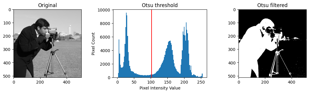
If you look at the filtered image (on the right-hand side of the plot), it seems to have achieved pretty good foreground/background segmentation…
How does the Otsu threshold filter work? Conceptually, the Otsu method involves splitting the histogram into two parts, at many different thresholds, and comparing different splits for how well they separate pixels into two classes, based on a specific numeric metric. The histogram, for each threshold, is split at the center one of the bin intervals.
The aim is to find which bin interval center gives a split that yields two classes of pixels which are maximally different from one another, by the aforementioned numeric metric. If we are lucky, this corresponds to pixels forming the background of the image vs pixels forming the foreground of the image.
Since the Otsu method relies on some of the mechanics of histograms, let’s
deconstruct the histogram in the center of the plot above, to see how the
method works. To perform this deconstruction, we can use the np.histogram()
function. We give it a flattened (1-D) image array (e.g. flattened with the
.ravel() method), and we give it a number of bins to use. Again, we will use
the sensible value of 128 bins. (Note: you could also use
ski.exposure.histogram() here, for similar results).
np.histogram() will return two arrays. The first is the pixel count within each bin, so in this case we will get 128 individual numbers, because there are 128 bins. We will call this array counts. These counts determine the height of the histogram over each bin. The first count is for the first bin, the second count is for the second bin, and so on, as we move along the \(x\)-axis from left to right.
The second array returned by np.histogram() contains the start point of each
bin (e.g. each \(x\)-axis interval within which we get the Pixel Count),
followed by the end-point of the last bin. We will call this array edges.
The size of each array will vary, based on the number of bins we ask NumPy to use to make the histogram:
# Get `counts` and `edges`.
counts, edges = np.histogram(camera.ravel(),
                             bins=128)
# Show counts.
counts
array([   2,  628, 5624, 3516, 1844, 1479, 1427, 1464, 1605, 2272, 3101,
       4955, 7451, 9584, 9191, 6119, 3754, 2452, 1677, 1288,  988,  885,
        901,  837,  796,  640,  602,  566,  582,  480,  456,  404,  382,
        398,  352,  316,  343,  350,  314,  312,  289,  324,  308,  314,
        296,  320,  304,  315,  343,  399,  410,  424,  414,  412,  484,
        495,  573,  632,  777,  861,  940, 1033, 1213, 1368, 1492, 1783,
       1951, 2164, 2392, 2610, 3001, 3338, 3911, 4233, 4340, 4759, 5196,
       5341, 5398, 5428, 5104, 4808, 4051, 3360, 2588, 2067, 1582, 1352,
       1186,  997,  860,  773,  706,  566,  569, 1877, 2709, 3980, 6792,
       6318, 7477, 6217, 5413, 8153, 7025, 6540, 5459, 3523, 1825, 1074,
       1713,  710,  316,  330,  472,  412,  324,  275,  157,  135,  201,
         66,   73,   95,  102,  128,  198,  564])
# Show `edges`.
edges
array([  0.  ,   1.99,   3.98,   5.98,   7.97,   9.96,  11.95,  13.95,
        15.94,  17.93,  19.92,  21.91,  23.91,  25.9 ,  27.89,  29.88,
        31.88,  33.87,  35.86,  37.85,  39.84,  41.84,  43.83,  45.82,
        47.81,  49.8 ,  51.8 ,  53.79,  55.78,  57.77,  59.77,  61.76,
        63.75,  65.74,  67.73,  69.73,  71.72,  73.71,  75.7 ,  77.7 ,
        79.69,  81.68,  83.67,  85.66,  87.66,  89.65,  91.64,  93.63,
        95.62,  97.62,  99.61, 101.6 , 103.59, 105.59, 107.58, 109.57,
       111.56, 113.55, 115.55, 117.54, 119.53, 121.52, 123.52, 125.51,
       127.5 , 129.49, 131.48, 133.48, 135.47, 137.46, 139.45, 141.45,
       143.44, 145.43, 147.42, 149.41, 151.41, 153.4 , 155.39, 157.38,
       159.38, 161.37, 163.36, 165.35, 167.34, 169.34, 171.33, 173.32,
       175.31, 177.3 , 179.3 , 181.29, 183.28, 185.27, 187.27, 189.26,
       191.25, 193.24, 195.23, 197.23, 199.22, 201.21, 203.2 , 205.2 ,
       207.19, 209.18, 211.17, 213.16, 215.16, 217.15, 219.14, 221.13,
       223.12, 225.12, 227.11, 229.1 , 231.09, 233.09, 235.08, 237.07,
       239.06, 241.05, 243.05, 245.04, 247.03, 249.02, 251.02, 253.01,
       255.  ])
Look at the first two values in the edges array; they form the interval for
the first bin. So the first bin interval runs from 0 up to but not including
1.99, the second interval runs between the next two values of 1.99 up to (not
including 3.98 and so on. The last two elements in the edges array are the
start and inclusive end of the last bin — in this case from 253.01 up to
and including 255.
Let’s state that again in a different way. Say there are \(n\) bins (here
128). For all bins from \(i = 0..n - 1\) (here \(i = 0..127\)), the start value is
edges[i]. For all bins but the last edges[i + 1] gives the exclusive
end of the bin. For the last bin (\(i = n - 2\)), the last value in edges
gives the inclusive end of the last bin.
Each value in counts is the count of pixel intensity values in camera
which fall within the corresponding interval. Let’s check this is correct by
Boolean indexing camera to see how many pixels fall within the first
interval (0 up to, not including 1.99):
# For the first bin interval.
camera[(camera >= 0) & (camera < 1.99)]
array([0, 1], dtype=uint8)
Sure enough there are two pixels in the interval, which corresponds to the first value in the counts array:
# The first value in the `counts` array.
counts[0]
np.int64(2)
The second interval (e.g. the next two edges values) runs from 1.99 up to (not including) 3.98. The second value of the counts array is 628, so there should be 628 pixels within this interval:
# The second value in `counts`.
counts[1]
np.int64(628)
Let’s manually get the pixels in camera which fall in this second bin interval:
# For the second bin interval.
camera[(camera >= 1.99) & (camera < 3.98)]
array([3, 3, 3, 3, 3, 3, 3, 3, 3, 3, 3, 3, 2, 3, 3, 3, 3, 3, 2, 3, 3, 3,
       3, 3, 3, 3, 3, 3, 2, 2, 3, 3, 3, 3, 3, 3, 3, 3, 3, 3, 3, 3, 3, 3,
       3, 3, 3, 3, 3, 3, 3, 3, 3, 3, 3, 3, 3, 3, 3, 3, 3, 3, 3, 3, 3, 3,
       3, 3, 3, 3, 3, 3, 3, 3, 3, 3, 3, 3, 3, 3, 3, 3, 3, 3, 3, 3, 3, 3,
       3, 3, 2, 3, 3, 3, 3, 3, 3, 3, 3, 3, 3, 3, 2, 3, 3, 3, 3, 3, 3, 3,
       3, 3, 3, 3, 3, 3, 3, 3, 3, 3, 3, 3, 3, 3, 3, 3, 3, 3, 3, 3, 3, 3,
       3, 3, 3, 3, 3, 3, 3, 3, 3, 3, 3, 3, 3, 3, 3, 3, 3, 3, 3, 3, 3, 3,
       3, 3, 3, 3, 3, 3, 3, 3, 3, 2, 2, 3, 3, 3, 3, 3, 3, 3, 3, 3, 3, 3,
       3, 3, 3, 3, 3, 3, 3, 3, 3, 3, 3, 3, 3, 3, 3, 3, 3, 3, 3, 3, 3, 3,
       3, 3, 3, 3, 3, 3, 3, 3, 3, 3, 3, 3, 3, 3, 3, 3, 3, 3, 3, 3, 3, 2,
       3, 3, 3, 3, 3, 3, 3, 3, 3, 3, 3, 3, 3, 3, 3, 3, 3, 3, 3, 3, 3, 3,
       3, 3, 3, 3, 3, 3, 3, 3, 3, 3, 3, 3, 3, 3, 3, 3, 3, 3, 3, 3, 3, 3,
       3, 3, 3, 3, 3, 3, 3, 3, 3, 3, 3, 3, 3, 3, 3, 3, 3, 3, 3, 3, 3, 3,
       3, 3, 3, 3, 3, 3, 3, 3, 3, 3, 3, 3, 3, 3, 3, 3, 3, 3, 3, 3, 3, 3,
       3, 3, 3, 3, 3, 3, 3, 3, 3, 2, 3, 3, 3, 3, 3, 3, 3, 3, 3, 3, 3, 3,
       3, 3, 3, 3, 3, 3, 3, 3, 3, 3, 3, 3, 3, 3, 3, 3, 3, 3, 3, 3, 3, 3,
       3, 3, 3, 3, 3, 3, 3, 3, 3, 3, 3, 3, 3, 3, 3, 3, 3, 3, 3, 3, 3, 3,
       3, 3, 3, 3, 3, 3, 3, 3, 3, 3, 3, 3, 3, 3, 3, 3, 2, 3, 3, 3, 3, 3,
       3, 3, 3, 3, 3, 3, 3, 3, 3, 3, 3, 3, 3, 3, 3, 3, 3, 3, 3, 3, 3, 3,
       3, 3, 3, 3, 3, 3, 3, 3, 3, 3, 3, 3, 3, 3, 3, 3, 3, 3, 3, 3, 3, 3,
       3, 3, 3, 2, 3, 3, 3, 3, 3, 3, 3, 3, 3, 3, 3, 3, 3, 3, 3, 3, 3, 3,
       3, 3, 3, 3, 3, 3, 3, 3, 3, 3, 3, 3, 3, 3, 3, 3, 3, 3, 3, 3, 3, 3,
       3, 3, 3, 3, 3, 3, 3, 3, 3, 3, 3, 3, 3, 3, 3, 3, 3, 3, 3, 3, 3, 3,
       3, 3, 3, 3, 3, 3, 3, 3, 3, 3, 3, 3, 3, 3, 3, 3, 3, 3, 3, 3, 3, 3,
       3, 3, 3, 3, 3, 3, 3, 3, 3, 3, 3, 3, 3, 3, 3, 3, 3, 3, 3, 3, 3, 3,
       3, 3, 3, 3, 3, 3, 3, 3, 3, 3, 3, 3, 3, 3, 3, 3, 3, 3, 3, 3, 3, 3,
       3, 3, 3, 3, 3, 3, 3, 3, 3, 3, 3, 3, 3, 2, 3, 3, 2, 3, 3, 2, 3, 2,
       2, 3, 2, 3, 3, 2, 3, 3, 3, 3, 3, 3, 3, 3, 3, 3, 3, 3, 3, 3, 3, 3,
       3, 3, 3, 3, 3, 2, 3, 3, 3, 3, 3, 3], dtype=uint8)
It certainly looks like there could be 600+ values in there! We don’t feel like counting, so let’s verify how many pixels there are in this bin interval using len():
# Count the pixels in the second bin interval.
len(camera[(camera >= 1.99) & (camera < 3.98)])
628
So, each adjacent pair of numbers in edges tells us the range of each bin
interval, and the corresponding value in counts tells us the height on the
histogram within that interval. The image below shows the first, second, third
and final (128th) interval in the edges array:

Ok, so we now have our deconstructed histogram. To implement the Otsu method, we next need to find the center of each bin interval (e.g. the middle point between the lower and higher number in each pair). Once we have the bin centers, we can use those to start splitting the histogram in two, to find the split that gives us the two most distinct groupings of pixels, on either side of the split. This is a simple calculation, we can get the start value of each bin interval with the following slicing operation:
# The first value of each bin interval.
edges[:-1]
array([  0.  ,   1.99,   3.98,   5.98,   7.97,   9.96,  11.95,  13.95,
        15.94,  17.93,  19.92,  21.91,  23.91,  25.9 ,  27.89,  29.88,
        31.88,  33.87,  35.86,  37.85,  39.84,  41.84,  43.83,  45.82,
        47.81,  49.8 ,  51.8 ,  53.79,  55.78,  57.77,  59.77,  61.76,
        63.75,  65.74,  67.73,  69.73,  71.72,  73.71,  75.7 ,  77.7 ,
        79.69,  81.68,  83.67,  85.66,  87.66,  89.65,  91.64,  93.63,
        95.62,  97.62,  99.61, 101.6 , 103.59, 105.59, 107.58, 109.57,
       111.56, 113.55, 115.55, 117.54, 119.53, 121.52, 123.52, 125.51,
       127.5 , 129.49, 131.48, 133.48, 135.47, 137.46, 139.45, 141.45,
       143.44, 145.43, 147.42, 149.41, 151.41, 153.4 , 155.39, 157.38,
       159.38, 161.37, 163.36, 165.35, 167.34, 169.34, 171.33, 173.32,
       175.31, 177.3 , 179.3 , 181.29, 183.28, 185.27, 187.27, 189.26,
       191.25, 193.24, 195.23, 197.23, 199.22, 201.21, 203.2 , 205.2 ,
       207.19, 209.18, 211.17, 213.16, 215.16, 217.15, 219.14, 221.13,
       223.12, 225.12, 227.11, 229.1 , 231.09, 233.09, 235.08, 237.07,
       239.06, 241.05, 243.05, 245.04, 247.03, 249.02, 251.02, 253.01])
…and we can get the second value of each bin interval with:
# The second value of each interval.
edges[1:]
array([  1.99,   3.98,   5.98,   7.97,   9.96,  11.95,  13.95,  15.94,
        17.93,  19.92,  21.91,  23.91,  25.9 ,  27.89,  29.88,  31.88,
        33.87,  35.86,  37.85,  39.84,  41.84,  43.83,  45.82,  47.81,
        49.8 ,  51.8 ,  53.79,  55.78,  57.77,  59.77,  61.76,  63.75,
        65.74,  67.73,  69.73,  71.72,  73.71,  75.7 ,  77.7 ,  79.69,
        81.68,  83.67,  85.66,  87.66,  89.65,  91.64,  93.63,  95.62,
        97.62,  99.61, 101.6 , 103.59, 105.59, 107.58, 109.57, 111.56,
       113.55, 115.55, 117.54, 119.53, 121.52, 123.52, 125.51, 127.5 ,
       129.49, 131.48, 133.48, 135.47, 137.46, 139.45, 141.45, 143.44,
       145.43, 147.42, 149.41, 151.41, 153.4 , 155.39, 157.38, 159.38,
       161.37, 163.36, 165.35, 167.34, 169.34, 171.33, 173.32, 175.31,
       177.3 , 179.3 , 181.29, 183.28, 185.27, 187.27, 189.26, 191.25,
       193.24, 195.23, 197.23, 199.22, 201.21, 203.2 , 205.2 , 207.19,
       209.18, 211.17, 213.16, 215.16, 217.15, 219.14, 221.13, 223.12,
       225.12, 227.11, 229.1 , 231.09, 233.09, 235.08, 237.07, 239.06,
       241.05, 243.05, 245.04, 247.03, 249.02, 251.02, 253.01, 255.  ])
Note
Last values of edges
Remember, the last value in edges (edges[-1]) is the inclusive end of
the last bin. edges[1:-1] give the exclusive ends of the other bins.
Check the numbers in these two arrays against the image above (of the bin intervals) to verify they are correct. To get the bin center points, we just take the average of each pair:
# Get the center of each bin.
bin_centers = (edges[1:] + edges[:-1]) / 2
bin_centers
array([  1.  ,   2.99,   4.98,   6.97,   8.96,  10.96,  12.95,  14.94,
        16.93,  18.93,  20.92,  22.91,  24.9 ,  26.89,  28.89,  30.88,
        32.87,  34.86,  36.86,  38.85,  40.84,  42.83,  44.82,  46.82,
        48.81,  50.8 ,  52.79,  54.79,  56.78,  58.77,  60.76,  62.75,
        64.75,  66.74,  68.73,  70.72,  72.71,  74.71,  76.7 ,  78.69,
        80.68,  82.68,  84.67,  86.66,  88.65,  90.64,  92.64,  94.63,
        96.62,  98.61, 100.61, 102.6 , 104.59, 106.58, 108.57, 110.57,
       112.56, 114.55, 116.54, 118.54, 120.53, 122.52, 124.51, 126.5 ,
       128.5 , 130.49, 132.48, 134.47, 136.46, 138.46, 140.45, 142.44,
       144.43, 146.43, 148.42, 150.41, 152.4 , 154.39, 156.39, 158.38,
       160.37, 162.36, 164.36, 166.35, 168.34, 170.33, 172.32, 174.32,
       176.31, 178.3 , 180.29, 182.29, 184.28, 186.27, 188.26, 190.25,
       192.25, 194.24, 196.23, 198.22, 200.21, 202.21, 204.2 , 206.19,
       208.18, 210.18, 212.17, 214.16, 216.15, 218.14, 220.14, 222.13,
       224.12, 226.11, 228.11, 230.1 , 232.09, 234.08, 236.07, 238.07,
       240.06, 242.05, 244.04, 246.04, 248.03, 250.02, 252.01, 254.  ])
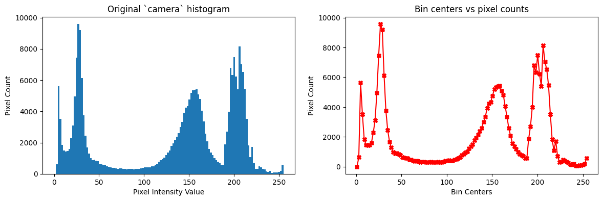
You’ll see that if we plot our bin_centers (\(x\)-axis) and our pixel counts (\(y\)-axis) we get something very much resembling the camera histogram, with 128 bins. Below the original camera histogram is shown on the left, and the plot of the bin_centers and counts arrays is shown on the right:
# Generate a plot.
plt.figure(figsize=(14, 4))
plt.subplot(1, 2, 1)
plt.hist(camera.ravel(), bins=128)
plt.xlabel('Pixel Intensity Value')
plt.ylabel('Pixel Count')
plt.title('Original `camera` histogram')
plt.subplot(1, 2, 2)
plt.plot(bin_centers, counts, color='red', marker='X')
plt.xlabel('Bin Centers')
plt.ylabel('Pixel Count')
plt.title('Bin centers vs pixel counts');
To implement the Otsu filter, we “split” the histogram into two sides, at a given bin center. We can think of this as creating two separate histograms. Here is a visualisation of splitting at the 50th bin center (which is centered on the pixel intensity value of 98.6). The location of the split is shown as a thick, dashed line:
# The 50th bin center value.
bin_centers[49]
np.float64(98.61328125)
# A function to visualise different threshold values.
def plot_bins_with_threshold(threshold_bin_number, legend=True, axis=True):
    plt.plot(bin_centers[:threshold_bin_number],
             counts[:threshold_bin_number],
             color='red',
             marker='X',
             label='Left Side Histogram')
    plt.plot(bin_centers[threshold_bin_number:],
             counts[threshold_bin_number:],
             color='green',
             marker='X',
             label='Right Side Histogram')
    plt.axvline(bin_centers[threshold_bin_number], color='black', label='Threshold',
                linestyle="--", linewidth=3)
    plt.xlabel('Bin Centers')
    plt.ylabel('Pixel Count')
    thresh_center = np.round(bin_centers[threshold_bin_number], 2)
    plt.title(f'Threshold Pixel Intensity = {thresh_center}')
    if legend == True:
        plt.legend(bbox_to_anchor=(1, 1))
    if axis == False:
        plt.xticks([])
        plt.yticks([]);

# Generate the plot.
plot_bins_with_threshold(49)
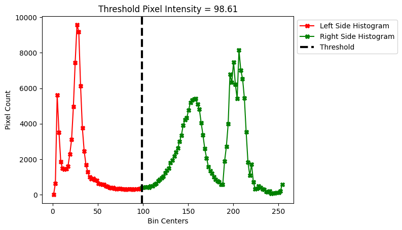
We now effectively have two histograms, the red one (below the 50th bin center; below a pixel intensity value of 98.6), and the green one (above the 50th bin center; above a pixel intensity value of 98.6).
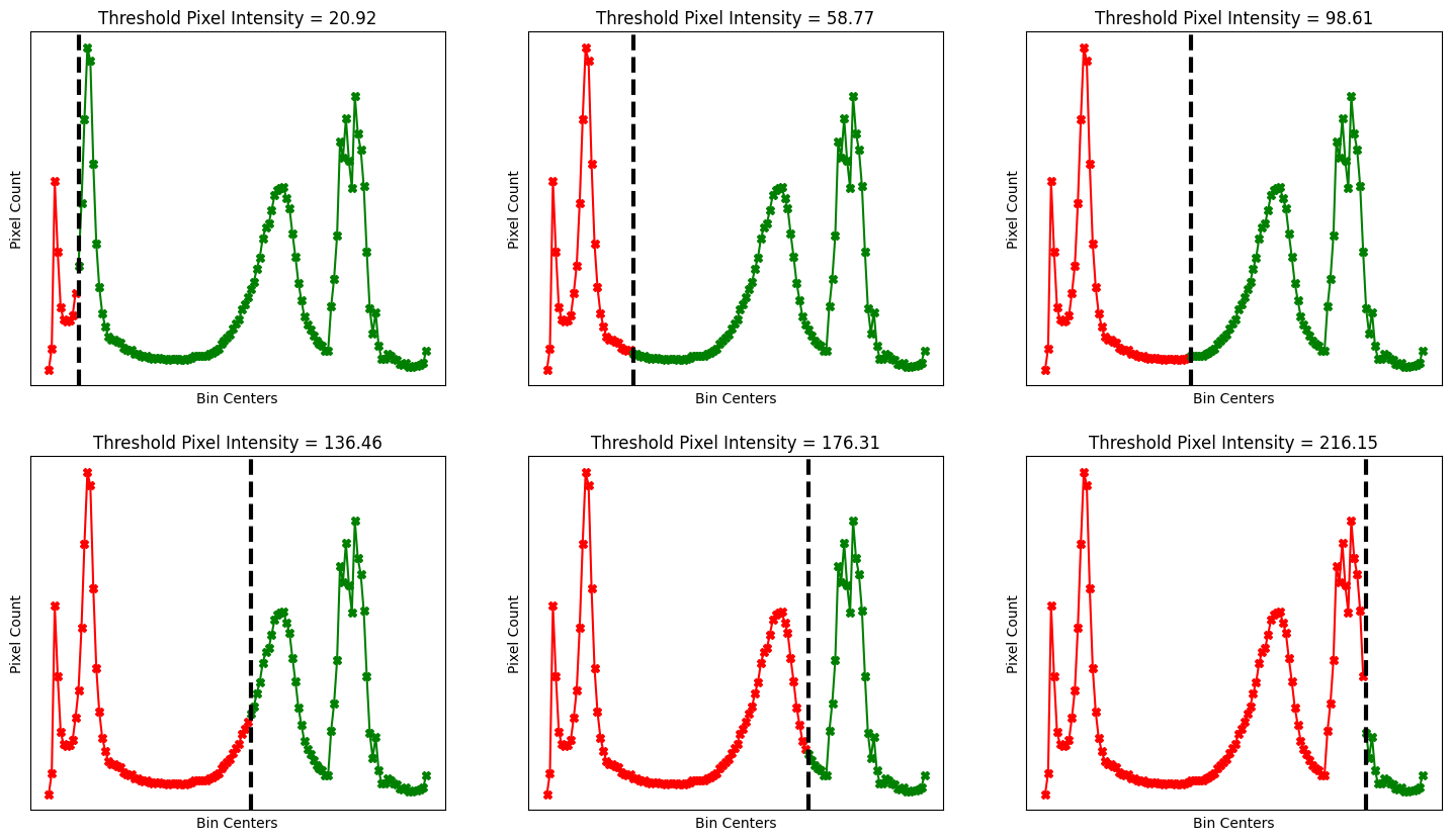
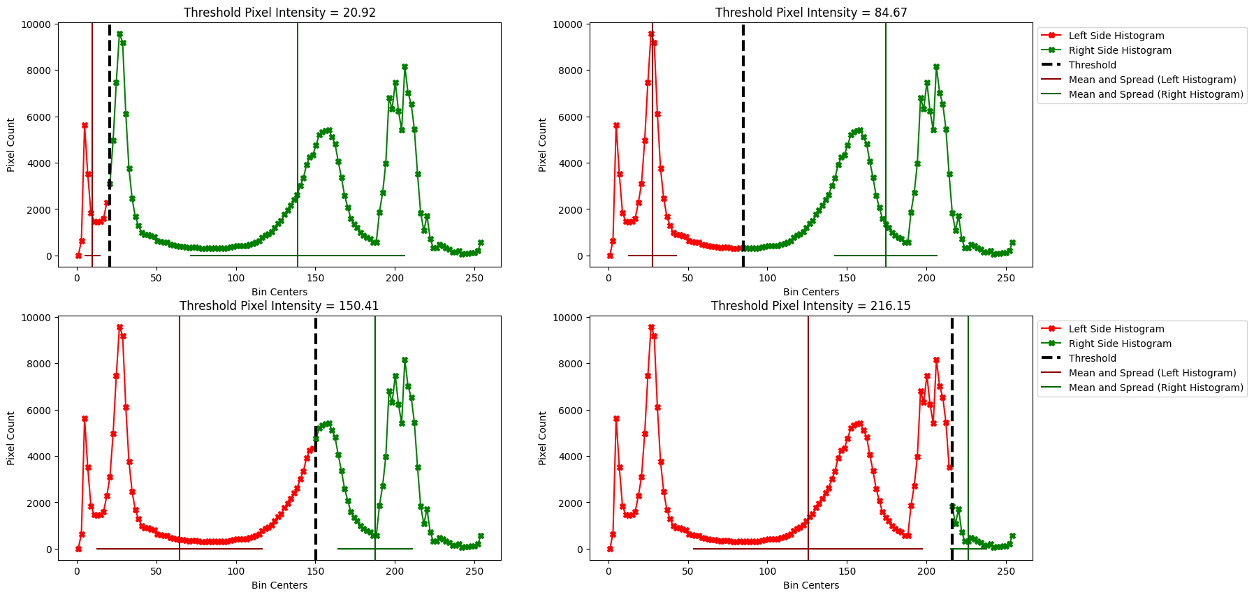
We can choose any bin center for the threshold, in fact, the Otsu filtering process will compare all possible thresholds/splits, comparing all of the bin centers. Multiple different splits are visualised below:
# Visualise multiple thresholds.
n_threshold_plots = 6
plt.figure(figsize=(18, 10))
for i, threshold_bin_num in enumerate(np.linspace(10, len(bin_centers)-20, num=n_threshold_plots).astype(int)):
    plt.subplot(2, int(n_threshold_plots/2), i+1)
    plot_bins_with_threshold(threshold_bin_num, legend=False, axis=False)
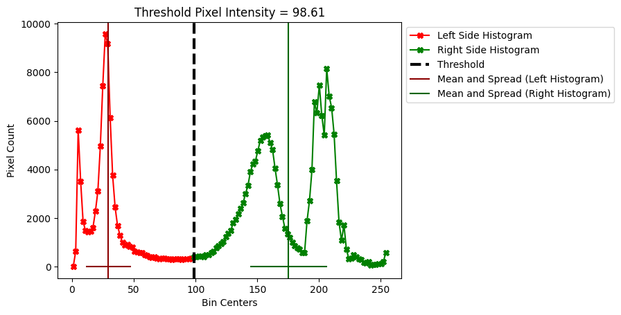
Once we have “split” the histogram, we calculate the mean of the pixel intensity values in the left-hand histogram, and the mean of the pixel intensity values in the right-hand histogram (e.g. either side of the split).
Then we calculate the sum of squared deviations (ssd) for each side of the histogram, each around its respective mean. This gives a metric of how “spread out” the values in each histogram are, around each mean.
It is this ssd metric which can allow us to select the “best” threshold; for giving distinct pixel classes…
The cell below defines a function which calculates the sum of the squared deviations, for a given histogram:
def ssd(counts, centers):
    """ Sum of squared deviations from mean """
    n = np.sum(counts)
    mean = np.sum(centers * counts) / n
    ssd = np.sum(counts * ((centers - mean) ** 2))
    return mean, ssd, n
Let’s use this function to calculate the mean and ssd of each histogram, when using the 50th bin center as the threshold:
# The mean and SSD for the left-hand histogram.
mean_below_50th_bin, ssd_below_50th_bin, n_below_50th_bin  = ssd(counts[:49], bin_centers[:49])
print("Mean of histogram below the 50th bin:", mean_below_50th_bin.round(2))
print("SSD of histogram  below the 50th bin:", ssd_below_50th_bin.round(2))
Mean of histogram below the 50th bin: 29.44
SSD of histogram  below the 50th bin: 27737445.29
# The mean and SSD for the right-hand histogram.
mean_above_50th_bin, ssd_above_50th_bin, n_above_50th_bin = ssd(counts[49:], bin_centers[49:])
print("Mean of histogram above the 50th bin:", mean_above_50th_bin.round(2))
print("SSD of histogram above the 50th bin:", ssd_above_50th_bin.round(2))
Mean of histogram above the 50th bin: 175.33
SSD of histogram above the 50th bin: 174551091.73
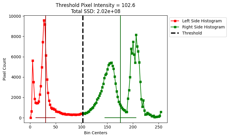
The cell below defines a convenience plotting function, the mean of each histogram is shown on the plot, as a vertical line in the same color as the histogram that it corresponds to (left or right). A horizontal line around each mean indicates the spread around that mean (FYI this spread has been converted back to the original scale of the plot, rather than the squared value of the ssd):
# A convenience plotting function.
def plot_thresh_mean_and_spread(threshold_bin_num, show_total_SSD=False, legend=True):
    plot_bins_with_threshold(threshold_bin_num, legend=legend)

    # Histogram 1
    color='red'
    mean_1, ssd_1, n_1 = ssd(counts[:threshold_bin_num], bin_centers[:threshold_bin_num])
    std_1 = np.sqrt(ssd_1/n_1)
    plt.axvline(mean_1, color='dark'+color, label=f'Mean and Spread (Left Histogram)')
    plt.hlines(10, mean_1 - std_1, mean_1 + std_1, color='dark'+color)

    # Histogram 2
    hist_number = 2
    color='green'
    mean_2, ssd_2, n_2 = ssd(counts[threshold_bin_num:], bin_centers[threshold_bin_num:])
    std_2 = np.sqrt(ssd_2/n_2)
    plt.axvline(mean_2, color='dark'+color, label=f'Mean and Spread (Right Histogram)')
    plt.hlines(10, mean_2 - std_2, mean_2 + std_2, color='dark'+color)

    if show_total_SSD == True:
        total_SSD = ssd_1 + ssd_2
        plt.title(f'Threshold Pixel Intensity = {bin_centers[threshold_bin_num].round(2)}\nTotal SSD: {total_SSD.round(2):.2e}')

# Add both means to the plot.
plot_thresh_mean_and_spread(49)
plt.legend(bbox_to_anchor=(1, 1));
Different threshold values change the mean and the spread (ssd) of each histogram. For each different split visualised below, pay attention to the width of the spread around each mean (e.g. the horizontal lines coming off the vertical line for each mean). This will let you see how the different splits influence the mean and the ssd of each histogram, when we compare the left histogram vs right histogram, for a given split.
Note
Spread, standard deviation and SSD
Bear in mind that we represent the spread around the mean in these plots as the standard deviation (SD) of the values either side of the split, around their respective means. The SD gives you an idea of the average spread of each of the two histograms.
However, remember that the actual metric used to evaluate the split is not the SD of the two histograms, but the sum of squared deviation (SSD). You can think of the SSD for each histogram, as the standard deviation (shown with the horizontal bar), squared (to give the variance) and then multiplied by the number of image values in the individual histogram. Thus even if the two histograms (left and right) have the same standard deviation, a tall histogram (with many values) will contribute a higher SSD than a shorter histogram (with fewer values). The metric used is the total SSD — that is the sum of the SSDs for the left and right histograms.
# Visualise multiple thresholds.
n_threshold_plots = 4
plt.figure(figsize=(18, 10))
for i, threshold_bin_num in enumerate(np.linspace(10, len(bin_centers)-20, num=n_threshold_plots).astype(int)):
    plt.subplot(2, int(n_threshold_plots/2), i+1)
    # Add both means to the plot.
    plot_thresh_mean_and_spread(threshold_bin_num, legend=False)
    if i%2 != 0:
        plt.legend(bbox_to_anchor=(1, 1));
In Otsu’s method, we want to find the threshold value which gives the minimum total ssd - e.g. the smallest value of the combined spread when we add together the ssd values for each histogram. This value corresponds to the maximum between pixel class variance, when comparing each side of the histogram.
In other words, the threshold value which gives the lowest combined ssd identifies two classes of pixels that are most different from each other, compared to other classes/splits we could choose, according the metric that the Otsu method cares about (the ssd).
You can think of this as finding a threshold which groups pixels such that the pixel values in each side of the “split” are clustered closely around their respective mean. In fact, it turns out minimizing the total ssd also has the effect that the distance between the means will be large, as well as giving a big separation between the pixels in each class as a result.
The cell below will find the threshold which gives the minimum combined ssd:
# An empty list to store all the `ssd` values, for all bin centers.
total_ssds = []

# Loop through the bin centers, compute the `ssd` of both
# histograms, for each threshold.
for bin_no in range(1, 128):
    left_mean, left_ssd, left_n = ssd(counts[:bin_no], bin_centers[:bin_no])
    right_mean, right_ssd, right_n = ssd(counts[bin_no:], bin_centers[bin_no:])

    # Calculate and store the total `ssd`, for the current threshold.
    total_ssds.append(left_ssd + right_ssd)

# Find the threshold which gives the smallest `ssd`. This is the Otsu threshold.
otsu_bin = np.argmin(total_ssds)
print('Otsu bin :', otsu_bin)
print('Otsu threshold:', bin_centers[otsu_bin])
Otsu bin : 51
Otsu threshold: 102.59765625
We can see that this is the same Otsu threshold we get from ski.filters.threshold_otsu(), when we use the same number of bins (128).
# Get the Otsu threshold from `skimage`.
ski.filters.threshold_otsu(camera,
                           nbins=128)
np.int64(102)
Here is the graph showing the Otsu threshold, the total ssd is shown, in scientific notation, in the title of the plot:
plot_thresh_mean_and_spread(otsu_bin, show_total_SSD=True)
The total ssd for the optimal Otsu threshold is an order of magnitude smaller than for some possible other threshold values. We show a different, much worse threshold below, which has a considerably larger total ssd (again, the total ssd is shown in the title of the plot):
# A much worse split.
plot_thresh_mean_and_spread(10, show_total_SSD=True)
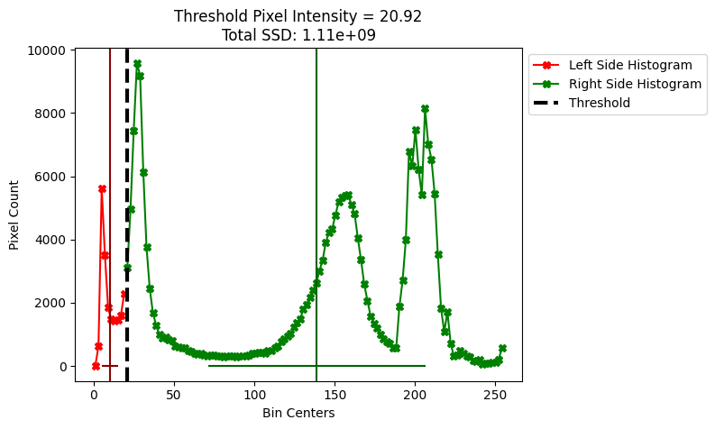
Compare the spreads on each plot by looking at the horizontal lines around the mean of each histogram. You can see that the spreads are much smaller for the Otsu threshold, than for the other, suboptimal threshold. The other threshold, because it has much worse between pixel-class variance than the Otsu threshold, gives much worse image segmentation, in terms of separating foreground from background:
# A bad segmentation, from the worse threshold value...
plt.imshow(camera < bin_centers[10]);
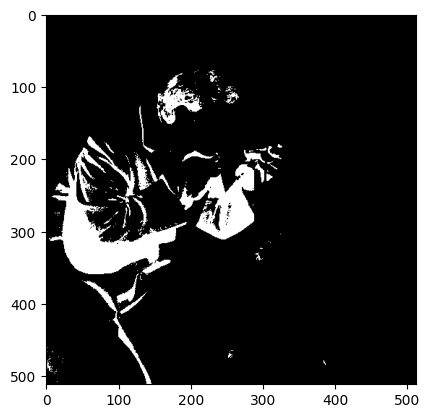
Admittedly that is quite a cool visual effect, but it is poor segmentation performance - it has not done a good job of splitting the foreground cameraman from the background. The ssds for multiple different thresholds are shown in the title of each plot below; the camera image filtered to the same threshold is shown to the right of each histogram plot:
# Visualise multiple thresholds, as well as filtering `camera` using those thresholds.
n_threshold_plots = 6
plt.figure(figsize=(24, 24))
thresholds=[10, 10, 60, 60, 120, 120]
for i in np.arange(n_threshold_plots):
    plt.subplot(int(n_threshold_plots/2), 2, i+1)
    if i % 2 == 0:
        plot_thresh_mean_and_spread(thresholds[i], show_total_SSD=True, legend=False)
    else:
        plt.imshow(camera < bin_centers[thresholds[i]])
        plt.title(f"Threshold Pixel Intensity: {bin_centers[thresholds[i]].round(2)}")
plt.subplots_adjust()
plt.tight_layout();
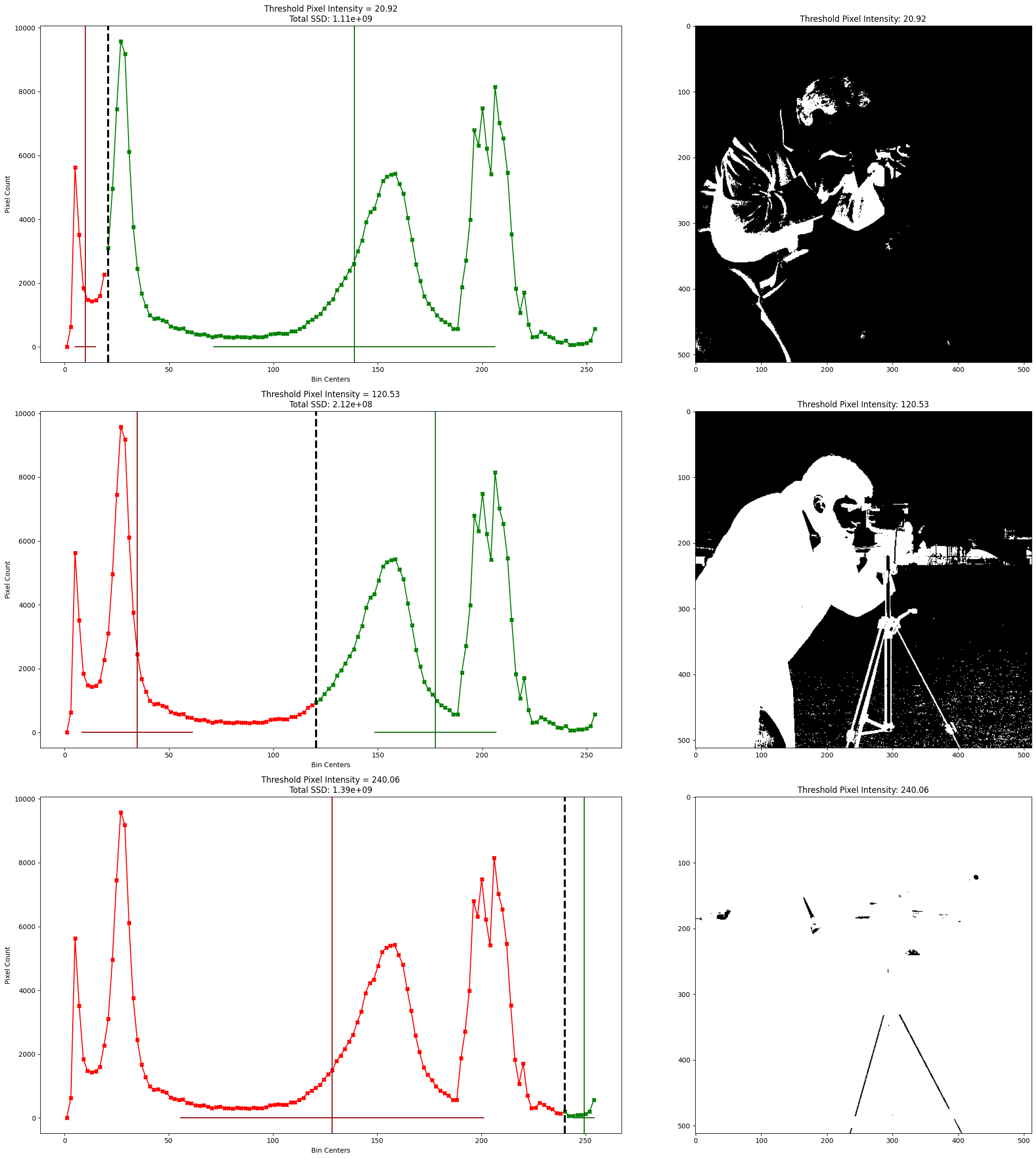
Remember: Otsu’s method finds the threshold which gives us the smallest sum of the ssd values, where we sum together the ssd value for each histogram. This identifies the two classes of pixels (one class in each histogram) which have the maximum between pixel-class variance, e.g. pixel classes which are optimally distinct from one another, when assessed with the ssd metric.
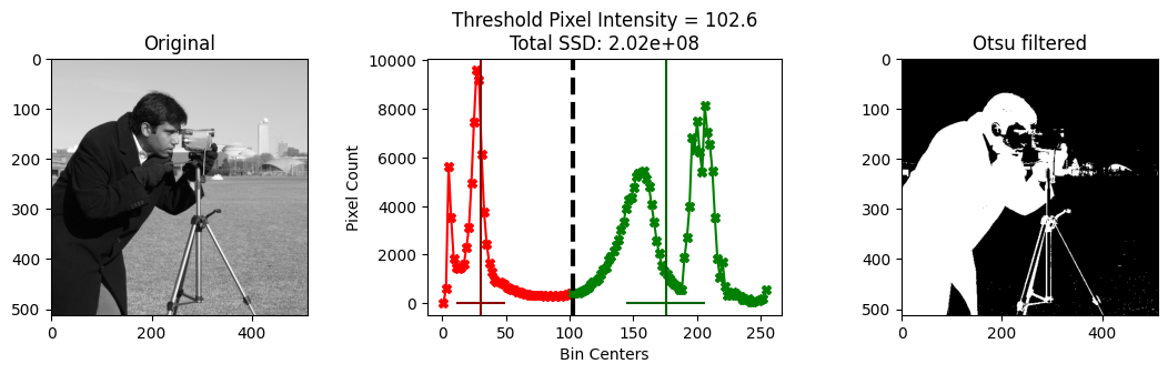
Compare the segmentation of the “best” Otsu threshold (shown below) to the poorer-performing thresholds shown on the right of the plot above - you will see substantially better foreground/background segmentation, from the optimal threshold:
# Show a plot of the whole Otsu filtering process.
plt.figure(figsize=(14, 3))
plt.subplot(1, 3, 1)
plt.imshow(camera)
plt.title('Original')
plt.subplot(1, 3, 2)
plot_thresh_mean_and_spread(otsu_bin, show_total_SSD=True, legend=False)
plt.subplot(1, 3, 3)
plt.imshow(camera_otsu_filtered)
plt.title('Otsu filtered')
plt.subplots_adjust();
To recap, Otsu’s method proceeds like this:
create the 1D histogram of image values, where the histogram has \(L\) bins. The histogram is \(L\) bin counts \(\vec{c} = [c_1, c_2, ... c_L]\), where \(c_i\) is the number of values falling in bin \(i\). The histogram has bin centers \(\vec{v} = [v_1, v_2, ..., v_L]\), where \(v_i\) is the image value corresponding to the center of bin \(i\);
for every bin number \(k \in [1, 2, 3, ..., L-1]\), divide the histogram at that bin to form a left histogram and a right histogram, where the left histogram has counts, centers \([c_1, ... c_k], [v_1, ... v_k]\), and the right histogram has counts, centers \([c_{k+1} ... c_L], [v_{k+1} .. v_L]\);
calculate the mean corresponding to the values in the left and right histogram:
\[\begin{split} \begin{align} n_k^{left} = \sum_{i=1}^{k} c_i \\ \mu_k^{left} = \frac{1}{n_k^{left}} \sum_{i=1}^{k} c_i v_i \\ n_k^{right} = \sum_{i={k+1}}^{L} c_i \\ \mu_k^{right} = \frac{1}{n_k^{right}} \sum_{i={k+1}}^{L} c_i v_i \end{align} \end{split}\]calculate the sum of squared deviations from the left and right means:
\[\begin{split} \begin{align} \mathrm{SSD}_k^{left} = \sum_{i=1}^{k} c_i (v_i - \mu_k^{left}) \\ \mathrm{SSD}_k^{right} = \sum_{i={k+1}}^{L} c_i (v_i - \mu_k^{right}) \\ \mathrm{SSD}_k^{total} = SSD_k^{left} + SSD_k^{right} \end{align} \end{split}\]find the bin number \(k\) that minimizes \(\mathrm{SSD}_k^{total}\):
\[ z = \mathrm{argmin}_k \mathrm{SSD}_k^{total} \]the binarizing threshold for the image is the value corresponding to this bin \(z\):
\[ t = v_z \]
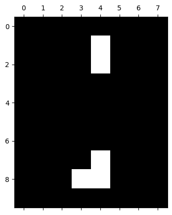
Exercise 20
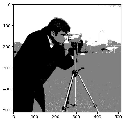
Your task now is to split camera into three distinct pixel classes, using threshold filtering. Here is your target image:
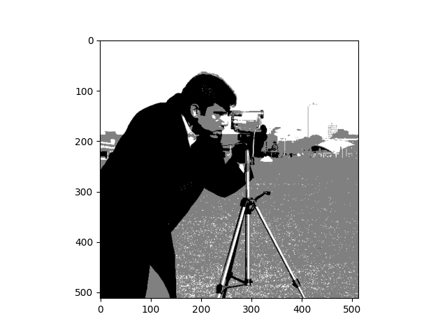
Roughly, in the target image, the sky has white pixels, the ground has gray pixels and the cameraman’s body has black pixels. Your final image should contain only the following np.unique() values:
array([0, 1, 2])
You can use a “by eye” method to decide your thresholds, from inspecting a histogram of camera. Or you can investigate using the skimage Otsu filter to get thresholds for more than two pixel classes…
# YOUR CODE HERE
Solution to Exercise 20
Inspecting the histogram by eye can get you quite far here. First, we plot the histogram of camera. We roughly identify low frequency regions which separate the modes of the distribution:
# Plot the histogram, and estimate, by eye thresholds.
plt.hist(camera.ravel(), bins=128)
plt.axvline(80, color='red', label='By eye threshold 1')
plt.axvline(190, color='darkred', label='By eye threshold 2')
plt.xlabel('Pixel Intensity Value')
plt.ylabel('Pixel Count')
plt.legend(bbox_to_anchor=(1, 1));
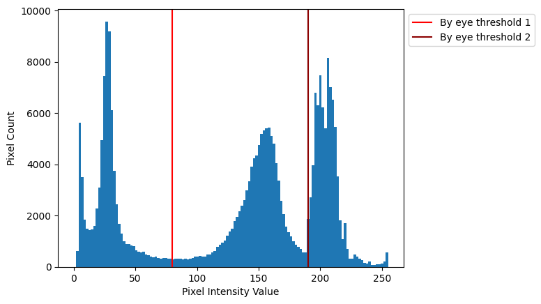
We chose 80 and 190, but you could get similar results with other nearby values:
# Save our estimated thresholds as separate variables.
by_eye_1 = 80
by_eye_2 = 190
We then use some Boolean indexing to:
Set values to the left of the lower threshold to 0.
Set values in between the thresholds to 1.
Set values to the right of the higher threshold to 2.
# Copy to avoid overwriting.
camera_region_solution = camera.copy()

# Set values to the left of the lower threshold to 0.
camera_region_solution[camera_region_solution < by_eye_1] = 0

# Set values in between the thresholds to 1.
camera_region_solution[(camera_region_solution >= by_eye_1) & (camera_region_solution <= by_eye_2)] = 1

# Set values to the right of the higher threshold to 2.
camera_region_solution[camera_region_solution > by_eye_2] = 2

# Show the result.
plt.imshow(camera_region_solution);
That gets us pretty close to the target image!
A less “back of the envelope” method is to use ski.filters.threshold_multiotsu() which is an adjustment of the Otsu method which, you guessed it, allows us to “split” a histogram into more than two parts.
The syntax is very straightforward, and the function returns a list of the threshold values:
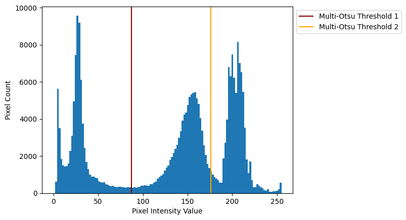
# Multi-Otsu filter.
otsu_cam3_solution = ski.filters.threshold_multiotsu(camera,
                                                     classes=3) # How many pixel classes?
# Show the thresholds.
otsu_cam3_solution
array([ 87, 176])
We plot the thresholds below:
# Plot the histogram, and the Multi-Otsu thresholds.
plt.hist(camera.ravel(), bins=128)
plt.axvline(otsu_cam3_solution[0], color='darkred', label='Multi-Otsu Threshold 1')
plt.axvline(otsu_cam3_solution[1], color='orange', label='Multi-Otsu Threshold 2')
plt.xlabel('Pixel Intensity Value')
plt.ylabel('Pixel Count')
plt.legend(bbox_to_anchor=(1, 1));
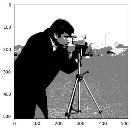
We can use Boolean indexing (as above) to set the pixel values according to the thresholds, by looping through the thresholds. But to be more elegant, we’ll use np.digitize to do the same job:
bins = np.concatenate([[0], otsu_cam3_solution, [np.max(camera) + 1.]])
bins
array([ 0., 87., 176., 256.])
# Digitize maps image values x to output values thus:
# - where bins[0] <= x < bins[1] -> output 0,
# - where bins[1] <= x < bins[2] -> output 1
# - where bins[2] <= x < bins[3] -> output 2.
camera_region_solution_multiotsu = np.digitize(camera, bins)

# Show the result.
plt.imshow(camera_region_solution_multiotsu);
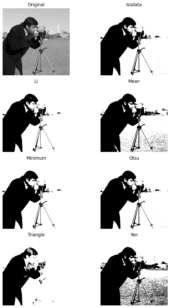
A useful trick, when thresholding in skimage to try to separate foreground and background, is to use the ski.filters.try_all_threshold() to test out all of the available thresholding methods, and visually inspect the results.
This function is both a filtering function and a plotting function. Behind the scenes it is using Matplotlib to generate the plots. Such is the utility of skimage being highly integrated with the rest of the Scientific Python eco-system.
We run the function in the cell below. The name of each thresholding method is shown as the title of each plot:
# Try all thresholding methods, and plot the results.
ski.filters.try_all_threshold(camera,
                              verbose=False, # Avoid clutter from printouts.
                              figsize=(12, 12))
plt.tight_layout();
Summary#
This page shows and explains threshold filtering using numpy, scipy and
skimage. On the next page we will look at kernel filtering,
where we modify pixel values based on the “local neighborhood” of surrounding
pixels.
References#
Gulati, J. (2024) NumPy for Image Processing. KDnuggets. Available from: https://www.kdnuggets.com/numpy-for-image-processing
Adapted from:
with further inspiration from Napari tutorial and skimage tutorials.