Filtering with kernels - the mean filter#
Note
This tutorial is adapted from “Image manipulation and processing using NumPy and SciPy” by Emmanuelle Gouillart and Gaël Varoquaux, and “scikit-image: image processing” by Emmanuelle Gouillart. Please see the References section at the end of the page for other sources and resources.
Footprints and pixel neighborhoods#
On the last page we filtered images based on a single threshold value, or based on multiple threshold values. Other filters work differently: they work by adjusting a given pixel’s value based on the value of other pixels which surround it, in a specified area. The mean filter is one such filter.
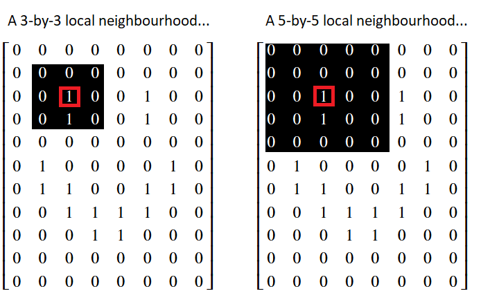
The mean filter is a local filter, because it alters a given pixel’s value based on the values of other pixels in the surrounding “local neighborhood”. The image below shows the pixel values in the smiley image array that we created on an earlier page. Two possible “local neighborhoods” are shown for a given pixel, which is highlighted in red. One neighborhood is 3-by-3, and the other is 5-by-5 — we could use either when using a local filter:
The values within a pixel’s local neighborhood affect the value that a local
filter calculates when applied to given pixel. The size and shape of the
“neighborhood” are up to the user. We can also refer to the neighborhood as
a “footprint” or “structuring element”. As we will see later, Scikit-image
favors the term “footprint”. For now, we will use the terms “footprint” and
“neighborhood” interchangeably to refer to some set of pixels that surround
a given pixel.
Note
Footprints are binary arrays defining neighborhood
Above we’ve show footprints that are squares of different sizes, but in general a footprint is a binary array defining the voxels in the pixel neighborhood, with True (1) meaning in the neighborhood, and False (0) meaning not in the neighborhood.
For example, instead of a square, we could use a cross-shaped footprint like this:
x_shape = np.array([[False, True, False],
                    [True,  True,  True],
                    [False, True, False]])
Note
Filtering with footprints and functions
The essence of footprint-based filtering is:
Define a local neighborhood with the footprint.
For each pixel in turn:
Place the footprint centered over the target pixel.
Use the footprint to identify the pixels in the image that are in the local neighborhood of the target pixel. Select these pixels.
Apply some function, such as
np.mean, to the selected pixel values, calculate a new value to replace the target pixel value in the output image.
We will call this method: footprint / function filtering.
The mean filter, as the name suggests, averages the pixel values within a footprint/neighborhood. To see this in action, let’s build a simple mean filter to filter an image array. First, we perform some imports, and change some defaults.
# Library imports.
import numpy as np
import matplotlib.pyplot as plt
import scipy.ndimage as ndi
import skimage as ski

# Set 'gray' as the default colormap
plt.rcParams['image.cmap'] = 'gray'

# Set NumPy precision to 2 decimal places
np.set_printoptions(precision=2)

# Custom functions for illustrations, hints, and to quickly report image
# attributes.
from skitut import show_attributes, hints
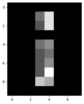
Next, we create the random_i image array:
# Create a grayscale image array.
random_i = np.array([[0, 0, 0, 0, 0, 0, 0, 0],
                     [0, 0, 0, 4, 8, 0, 0, 0],
                     [0, 0, 0, 3, 8, 0, 0, 0],
                     [0, 0, 0, 0, 0, 0, 0, 0],
                     [0, 0, 0, 4, 5, 0, 0, 0],
                     [0, 0, 0, 3, 4, 0, 0, 0],
                     [0, 0, 0, 3, 5, 0, 0, 0],
                     [0, 0, 0, 3, 9, 0, 0, 0],
                     [0, 0, 0, 7, 6, 0, 0, 0],
                     [0, 0, 0, 0, 0, 0, 0, 0]])
print(random_i)
plt.imshow(random_i);
[[0 0 0 0 0 0 0 0]
 [0 0 0 4 8 0 0 0]
 [0 0 0 3 8 0 0 0]
 [0 0 0 0 0 0 0 0]
 [0 0 0 4 5 0 0 0]
 [0 0 0 3 4 0 0 0]
 [0 0 0 3 5 0 0 0]
 [0 0 0 3 9 0 0 0]
 [0 0 0 7 6 0 0 0]
 [0 0 0 0 0 0 0 0]]
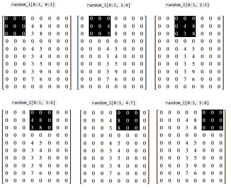
Let’s use some indexing to go for a walk through the neighborhoods
(footprints) in this array. As above, we’ll use a simple 3 by 3 pixel square
as the footprint — thus we treat each (3,3) set of pixels as
a separate neighborhood. For now, we only walk through the neighborhoods at
the “top” of the array. We will start our “walk” in the top-left corner of the
array, so that each 3-by-3 slice is centered on a pixel in the second row of
the image:
# Pixel values in the first neighborhood.
i_row_start, i_col_start = 0, 0
i_row_end, i_col_end = 3, 3
random_i[i_row_start:i_row_end, i_col_start:i_col_end]
array([[0, 0, 0],
       [0, 0, 0],
       [0, 0, 0]])
# The second neighborhood.
i_row_start, i_col_start = 0, 1
i_row_end, i_col_end = 3, 4
random_i[i_row_start:i_row_end, i_col_start:i_col_end]
array([[0, 0, 0],
       [0, 0, 4],
       [0, 0, 3]])
# The third neighborhood.
i_row_start, i_col_start = 0, 3
i_row_end, i_col_end = 3, 6
random_i[i_row_start:i_row_end, i_col_start:i_col_end]
array([[0, 0, 0],
       [4, 8, 0],
       [3, 8, 0]])
Obviously, this “walk” is more efficient in a for loop:
for i in range(6):
    i_row_start, i_col_start = 0, i
    i_row_end, i_col_end = 3, i+3
    print(f"\nrandom_i[{i_row_start}:{i_row_end}, {i_col_start}:{i_col_end}]\n")
    print(random_i[i_row_start:i_row_end, i_col_start:i_col_end])
random_i[0:3, 0:3]

[[0 0 0]
 [0 0 0]
 [0 0 0]]

random_i[0:3, 1:4]

[[0 0 0]
 [0 0 4]
 [0 0 3]]

random_i[0:3, 2:5]

[[0 0 0]
 [0 4 8]
 [0 3 8]]

random_i[0:3, 3:6]

[[0 0 0]
 [4 8 0]
 [3 8 0]]

random_i[0:3, 4:7]

[[0 0 0]
 [8 0 0]
 [8 0 0]]

random_i[0:3, 5:8]

[[0 0 0]
 [0 0 0]
 [0 0 0]]
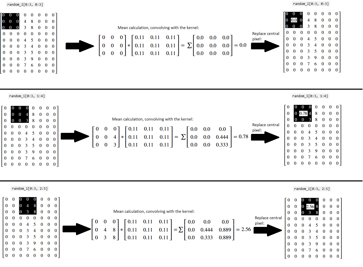
We can visualise the “walk” we have just taken, with prettier graphics — (you may want to right click on these images and open them in a new tab/window, for easier viewing):
Now, imagine we calculate the mean within each of these neighborhoods (footprints) - the mean of the pixel values within each footprint is shown below with the image of each indexing operation:
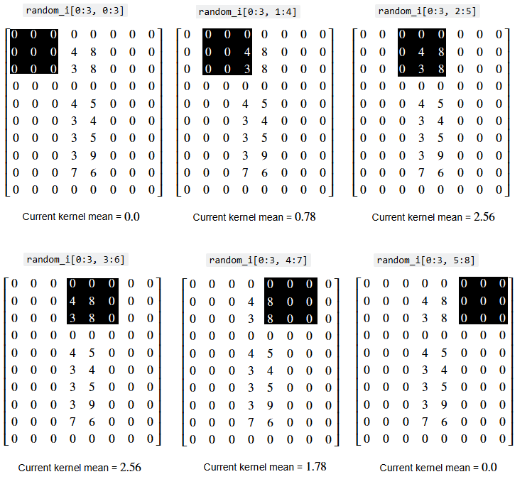
…and now further imagine that we replace the central pixel value of the 3-by-3 footprint with the mean of all the values in the footprint. The image below shows the central value being replaced with the mean with each footprint:
![]()
This is how the mean filter operates:
Define our footprint (e.g. our pixel neighborhood size and shape).
For each pixel:
Center our footprint on the given pixel.
Replace the value of the central pixel with the mean of the pixels in the neighborhood.
The illustrations above only show the footprint proceeding through the pixels at the “top” of the array. In reality, filtering operations are applied to every pixel in the image. You can think of this as the footprint “walking” through the entire array, being centered on one pixel at a time.
Astute readers might ask “what happens near the edges of the array? If we center our footprint on a pixel in the last column or row, won’t part of the footprint ‘fall off’ the edge of the array?’”:
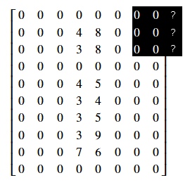
Indeed, we need a strategy for this. There are actually many options for how a footprint should behave at the edges of an image array - we could “pad” the footprint elements that fall outside of the image with 0 values, for instance. Or we could duplicate values from the pixels at the edge of the array, to fill in footprint elements that fall outside of the array. As we will see below, we will need a strategy like this for estimating the off-image values for the kernel filter methods.
However, for the “footprint” filters that we are considering here, the most obvious strategy is simply to clip the footprint at the edges, ignoring the part of the footprint that has fallen off the sides of the image. So, for example, in the illustration above, where the footprint has gone over the edge, we take the footprint to be only the part that remains covering the image. Thus, in the illustration, the effective footprint at the edge will be a 3 row by 2 column footprint.
Let us return to the implementation of a footprint filter. In general it looks like the illustration below, as we move the footprint to be centered on each pixel, select the image pixels within the footprint (remembering to clip at the edges), and apply our function to the footprint-selected pixels.
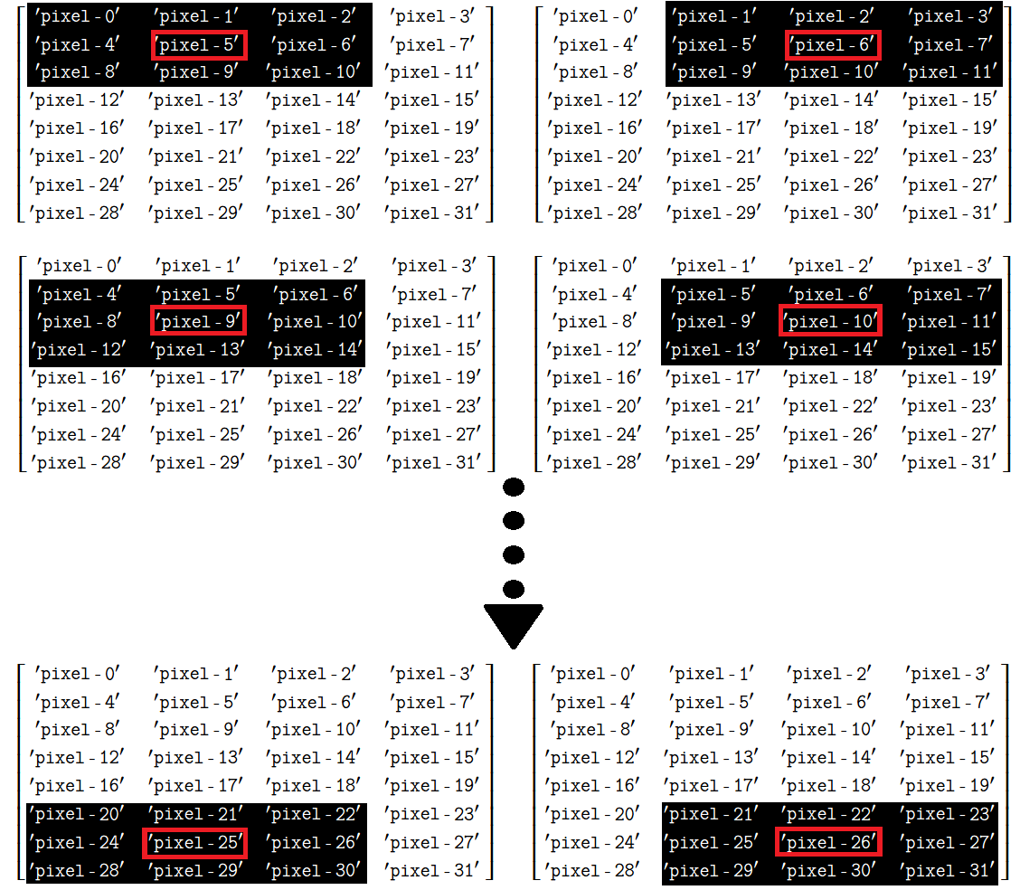
The cell below defines a function that will apply this mean footprint, step-by-step in a for loop, to the whole image array. Where the footprint falls off the sides of the image, we clip the footprint to fit inside the image.
# A function to apply our crude footprint / mean algorithm.
def three_by_three_mean_footprint(image):

    # Get the image shape.
    n_rows, n_cols = image.shape

    # Create an empty image array (for the result of the
    # filtering operation)
    filtered_image = np.zeros(image.shape)

    # Loop through the pixels and get the mean within each footprint.
    for i in range(n_rows):
        for j in range(n_cols):
            # Find the coordinates of the image pixels under the footprint.
            # Previous row to current, or 0 if above image.
            row_start = max(0, i - 1)
            # Previous column to current, or 0 if to right of image.
            col_start = max(0, j - 1)
            # Exclusive stop; 2 rows down, or n_rows if below image.
            row_end = min(n_rows, i + 2)
            # Exclusive stop; 2 rows across, or n_cols if left of image.
            col_end = min(n_cols, j + 2)
            # Index out part of image under footprint.
            selected = image[row_start:row_end, col_start:col_end]
            # Take mean.
            filtered_image[i, j] = np.mean(selected)
    return filtered_image
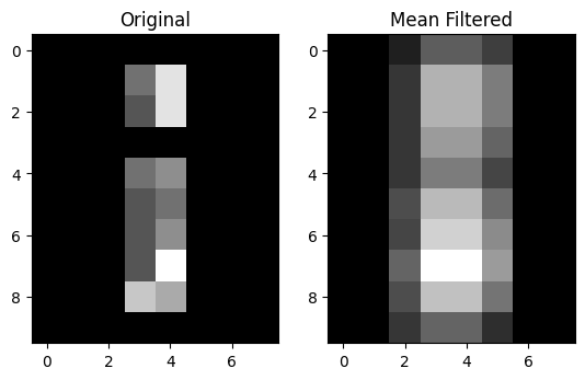
Let’s apply our crude footprint / mean filter to the image array, and compare it to the original image array:
# Apply our mean filtering function.
mean_filtered_i = three_by_three_mean_footprint(random_i)

# Show the original array and the filtered array, from the
# "raw" NumPy perspective.
print(f"Original:\n\n {random_i}")
print(f"\nCrude Mean filter:\n\n {mean_filtered_i}")

# Plot both arrays.
plt.subplot(1,2,1)
plt.imshow(random_i);
plt.title('Original')
plt.subplot(1,2,2)
plt.imshow(mean_filtered_i)
plt.title("Crude Mean Filter");
Original:

 [[0 0 0 0 0 0 0 0]
 [0 0 0 4 8 0 0 0]
 [0 0 0 3 8 0 0 0]
 [0 0 0 0 0 0 0 0]
 [0 0 0 4 5 0 0 0]
 [0 0 0 3 4 0 0 0]
 [0 0 0 3 5 0 0 0]
 [0 0 0 3 9 0 0 0]
 [0 0 0 7 6 0 0 0]
 [0 0 0 0 0 0 0 0]]

Crude Mean filter:

 [[0.   0.   0.67 2.   2.   1.33 0.   0.  ]
 [0.   0.   0.78 2.56 2.56 1.78 0.   0.  ]
 [0.   0.   0.78 2.56 2.56 1.78 0.   0.  ]
 [0.   0.   0.78 2.22 2.22 1.44 0.   0.  ]
 [0.   0.   0.78 1.78 1.78 1.   0.   0.  ]
 [0.   0.   1.11 2.67 2.67 1.56 0.   0.  ]
 [0.   0.   1.   3.   3.   2.   0.   0.  ]
 [0.   0.   1.44 3.67 3.67 2.22 0.   0.  ]
 [0.   0.   1.11 2.78 2.78 1.67 0.   0.  ]
 [0.   0.   1.17 2.17 2.17 1.   0.   0.  ]]
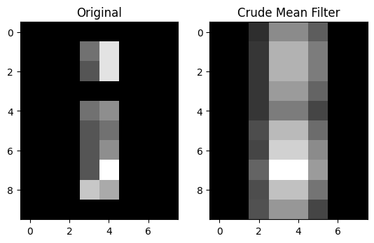
We can see that some of the non-black (non-zero) pixel intensity values have been “spread around” to neighboring pixels, which is unsurprising, given what we know about how this operation works. We have literally, for each given pixel, “averaged out” between the pixels in the 3-by-3 neighborhood around the pixel. This is a crude footprint / mean filter, intended to show the foundational principles of filtering via a footprint. There other ways to implement mean filters, however, to which we will come to in the next section.
Exercise 21
For this exercise, you should build a function which filters an image using a 3-by-3 footprint, like we did above. Your function should “walk” the 3-by-3 footprint through an image array, clipping the footprint at the image edges, as we did above.
However, the function you apply within the footprint should do something
different to the mean we implemented earlier. Your function will do something
dark, something illegal (or perhaps impolite, by the standards of skimage
dtype conventions)…
It should replace the central pixel value with the negative sum of the
values under the footprint (e.g. add the values under the footprint to give
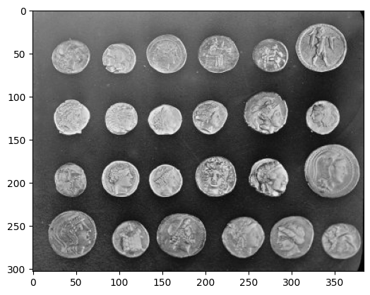
the sum, and then make the sum negative). You should apply this to the coins
image from ski.data. Here is the original image:
coins = ski.data.coins()
show_attributes(coins)
plt.imshow(coins)
Type: <class 'numpy.ndarray'>
dtype: uint8
Shape: (303, 384)
Max Pixel Value: 252
Min Pixel Value: 1
<matplotlib.image.AxesImage at 0x7ffb5e0e42d0>
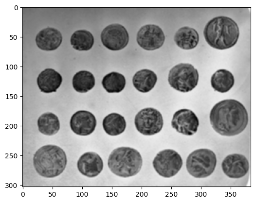
Here is how your image should look, after applying the negative sum filter, with a 3-by-3 footprint:

This operation will create some non-standard floating point pixel values - in
the sense that they are not between -1 and 1. You should rescale_intensity()
to ensure your image has the follow (legal!) attributes:
Type: <class 'numpy.ndarray'>
dtype: float64
Shape: (303, 384)
Max Pixel Value: 1.0
Min Pixel Value: -1.0
DO NOT ADJUST ANY OF THE FUNCTIONS USED ABOVE WHEN MAKING YOUR FUNCTION. Try to do this from scratch, clearly thinking about what you need to do.
# YOUR CODE HERE
def three_by_three_negative_sum_footprint():
    ...
Solution to Exercise 21
Whilst we told you not to adjust the function from above, obviously you function needs to do something similar to the function from above. So that was a rule for you, not for us ;)
Here we have adjusted the function to take the negative sum of the footprint
elements, rather than the mean. We also rescale_intensity() in the final
line, to ensure pixel values fall in a typical range, for the float64
dtype:
def three_by_three_negative_sum_footprint_solution(image):

    # Convert to float `dtype`.
    image = np.array(image,
                     dtype=float)

    # Get the image shape.
    n_rows, n_cols = image.shape

    # Create an empty image array (for the result of the
    # filtering operation)
    filtered_image = np.zeros(image.shape)

    # Loop through the pixels and get the negative sum within each footprint.
    for i in range(n_rows):
        for j in range(n_cols):
            row_start = max(0, i - 1)
            col_start = max(0, j - 1)
            row_end = min(n_rows, i + 2)
            col_end = min(n_cols, j + 2)
            footprint = image[row_start:row_end, col_start:col_end].copy()
            # Take the negative sum.
            filtered_image[i, j] = -np.sum(footprint)
    # Rescale to ensure legal pixel values.
    return ski.exposure.rescale_intensity(filtered_image, out_range="float64")
We reload in the coins image, to which to apply our new filter:
# Load in and show the `coins` image.
coins_solution = ski.data.coins()
plt.imshow(coins_solution);
We then apply our filter, replacing the value of the central pixel in each footprint with negative sum of the value of all the pixels under the footprint:
# Filter and show...
neg_sum_filter_coins = three_by_three_negative_sum_footprint_solution(
    coins_solution)
plt.imshow(neg_sum_filter_coins);
Here are the attributes of the somewhat ghostly, filtered image:
show_attributes(neg_sum_filter_coins)
Type: <class 'numpy.ndarray'>
dtype: float64
Shape: (303, 384)
Max Pixel Value: 1.0
Min Pixel Value: -1.0
Mean filtering with skimage#
ski.filters.rank.mean() implements a footprint / mean filter very much like
our crude version above. We supply a footprint array with which to “walk”
through the image, centering the footprint on every pixel, and modifying that
central pixel’s value based on the values of the other pixels in its
neighborhood, with the size and shape of the neighborhood being defined by the
footprint.
Inspecting the skimage documentation will reveal that the format expected
for the footprint should be “the [pixel] neighborhood expressed as an
ndarray of 1’s and
0’s.”.
We will use np.ones() to generate an array in this format. We use a (9, 9)
footprint to achieve a stronger visual effect:
# A "footprint" to pass to `skimage`.
footprint_9_by_9 = np.ones((9, 9))
footprint_9_by_9
array([[1., 1., 1., 1., 1., 1., 1., 1., 1.],
       [1., 1., 1., 1., 1., 1., 1., 1., 1.],
       [1., 1., 1., 1., 1., 1., 1., 1., 1.],
       [1., 1., 1., 1., 1., 1., 1., 1., 1.],
       [1., 1., 1., 1., 1., 1., 1., 1., 1.],
       [1., 1., 1., 1., 1., 1., 1., 1., 1.],
       [1., 1., 1., 1., 1., 1., 1., 1., 1.],
       [1., 1., 1., 1., 1., 1., 1., 1., 1.],
       [1., 1., 1., 1., 1., 1., 1., 1., 1.]])
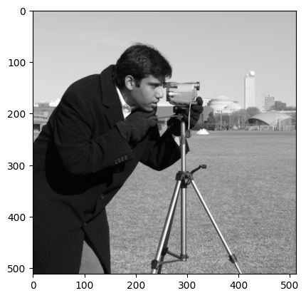
We will use it to filter the stalwart camera image:
# Import and show the `camera` image.
camera = ski.data.camera()
plt.imshow(camera);
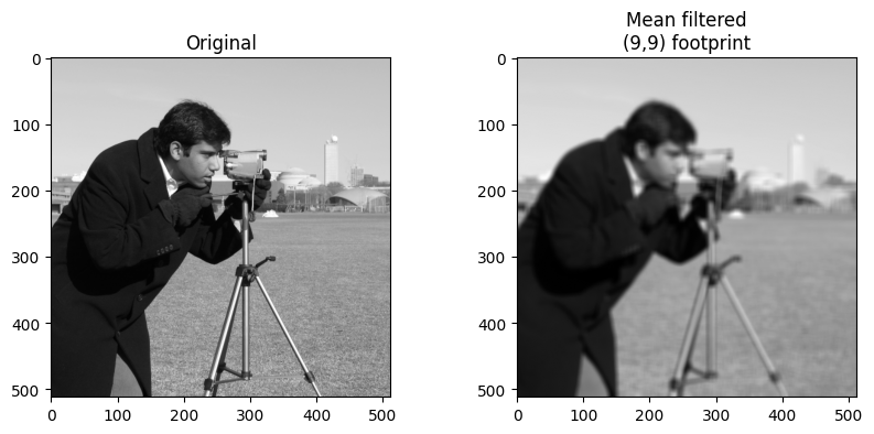
Below, we apply the mean filter, using the footprint_9_by_9 array as the
footprint. At each pixel, Scikit-image will place the footprint over the
pixel, select the values in the image with a corresponding 1 (or True) in the
footprint, and apply the mean operation to those values.
# Mean filter the `camera` image with `skimage`
mean_filtered_camera = ski.filters.rank.mean(camera,
                                             footprint=footprint_9_by_9)

# Plot both image to compare
plt.figure(figsize=(10, 4))
plt.subplot(1, 2, 1)
plt.title('Original')
plt.imshow(camera)
plt.subplot(1, 2, 2)
plt.title('Mean filtered\n(9,9) footprint')
plt.imshow(mean_filtered_camera);
Filtering with kernels#
We have so far seen filtering with footprints. We use a footprint array to specify the local neighborhood for any pixel. Then for each pixel, we apply the footprint at that pixel, to select the local pixels, and use some function, such as the mean, to calculate a single value from the neighboring pixels. This is the value at that pixel in the output image.
As you saw above, we call this footprint / function filtering.
Another, faster but less general way of applying local filters is by *applying a kernel.
Remember that a footprint is a binary array defining the neighborhood that defines which pixel values we consider as the neighborhood. For mean filtering, for example, we place the footprint over each pixel of the image, to define the neighboring values of the pixel, then apply an operation — taking the mean — to calculate the new pixel value.
A kernel is like a footprint array, but where the values of the array, instead of being binary (0 or 1), contain the weights to apply to the corresponding pixel in the neighborhood.
We generate the new filtered value by multiplying the kernel values by their corresponding pixels, and summing the result.
This should be come clear as the page progresses.
As for footprints, we “walk” a kernel across our whole image, centering it on every pixel, then apply the kernel weights to their corresponding pixel values, and sum to produce the new pixel value.
Let’s implement a mean filter, using a kernel. Obviously, we start with our kernel (a footprint with weights). First, we define the kernel shape:
# Define our kernel shape.
kernel_shape = (3, 3)
We’ll start the kernel as a suitably shape array of ones:
mean_kernel = np.ones(kernel_shape)
# Number of pixels in the kernel.
n = np.prod(kernel_shape)
n
np.int64(9)
Of course, in this case, where we’ve started with an array of all ones, we could also do this:
# Number of pixels in the kernel.
n = np.sum(mean_kernel)
n
np.float64(9.0)
A kernel is a footprint with weights. For a mean filter, the weights throughout the kernel should be \(\frac{1}{n}\), where \(n\) is the number of elements in our kernel, In our case this is \(\frac{1}{9}\) = 0.11:
mean_kernel = mean_kernel * 1 / n
mean_kernel
array([[0.11, 0.11, 0.11],
       [0.11, 0.11, 0.11],
       [0.11, 0.11, 0.11]])
Our purpose is to take the mean of the values under the kernel, so how does a 3-by-3 kernel filled with \(\frac{1}{n}\) help us?
Well, this value can be used to find the mean (duh!)…we’ll show this quickly using just four random values:
x = np.array([10, 21, 3, 45])
np.mean(x)
np.float64(19.75)
If we multiply each value by \(\frac{1}{n}\) and then take the sum of those values, we get…
n = len(x)
div_by_n = x * 1 / n
np.sum(div_by_n)
np.float64(19.75)
To belabor the point mathematically — write our vector (1D array) above as
\(\vec{x}\). Write the sum operation as \(\sum\). Then the mean of \(\vec{x}\)
is given by:
And we can do exactly the same thing with the mean_kernel we made above. We can use the scipy.ndimage.correlate() function to achieve this with maximum computational efficiency (relative to the crude method we used above). This function involves “moving a […] kernel over [an] image and computing the sum of products at each location”. This means we:
Center the kernel on given array pixel in the original image.
Multiply the array pixel values covered by the kernel with the elements in the kernel (in this case every kernel element value is \(\frac{1}{9}\)).
Get the sum of those products (e.g. add them all together to produce a single value).
Replace the central array pixel value in the original image with the single value we just computed.
Because we are using a mean kernel, this operation will, shockingly, return the mean of values under the kernel. This process is illustrated below for three kernel locations - (once more you may want to right click on these images and open them in a new tab/window, for easier viewing):
Now, let’s apply this kernel to every pixel in the image array:
# A new import.
import scipy.ndimage as ndi

# Filter
mean_filtered_random_i_via_sp = ndi.correlate(input=random_i,
                                              weights=mean_kernel,
                                              output=float) # Output `dtype`

# Show the original image array, and the mean filtered image array
print(f"Original:\n\n {random_i}")
print(f"\nMean filter:\n\n {mean_filtered_random_i_via_sp}")
plt.subplot(1, 2, 1)
plt.imshow(random_i)
plt.title("Original")
plt.subplot(1, 2, 2)
plt.title('Mean Filtered')
plt.imshow(mean_filtered_random_i_via_sp);
Original:

 [[0 0 0 0 0 0 0 0]
 [0 0 0 4 8 0 0 0]
 [0 0 0 3 8 0 0 0]
 [0 0 0 0 0 0 0 0]
 [0 0 0 4 5 0 0 0]
 [0 0 0 3 4 0 0 0]
 [0 0 0 3 5 0 0 0]
 [0 0 0 3 9 0 0 0]
 [0 0 0 7 6 0 0 0]
 [0 0 0 0 0 0 0 0]]

Mean filter:

 [[0.   0.   0.44 1.33 1.33 0.89 0.   0.  ]
 [0.   0.   0.78 2.56 2.56 1.78 0.   0.  ]
 [0.   0.   0.78 2.56 2.56 1.78 0.   0.  ]
 [0.   0.   0.78 2.22 2.22 1.44 0.   0.  ]
 [0.   0.   0.78 1.78 1.78 1.   0.   0.  ]
 [0.   0.   1.11 2.67 2.67 1.56 0.   0.  ]
 [0.   0.   1.   3.   3.   2.   0.   0.  ]
 [0.   0.   1.44 3.67 3.67 2.22 0.   0.  ]
 [0.   0.   1.11 2.78 2.78 1.67 0.   0.  ]
 [0.   0.   0.78 1.44 1.44 0.67 0.   0.  ]]
The result is very similar to that obtained by our crude mean filter. It’s similar, not identical, because the mathematics of applying the kernel at the edges, do not easily allow us to do what we did with the footprint / function method. As you remember, the footprint method immediately suggests we clip the footprint at the edges. This is not easily done with with the kernel methods, so we need instead (and internally) to expand the image with estimated edge pixels, before applying the kernel. You will see more on this below, but for now, let us confirm the results are similar, but not the same, using values rounded to 2 decimal places.
You can see that the values differ only near the top and bottom edges of the
image. ndi.correlate() offers several options for dealing with pixels at the
edge of the array (e.g. those pixels for which the kernel “falls off” the edge
of the image). Here are the options, from the
documentation;
we can choose an option by specifying the mode argument to ndi.correlate
(e.g. mode = 'constant' etc.):
mode : {'reflect', 'constant', 'nearest', 'mirror', 'wrap'}, optional
    The `mode` parameter determines how the input array is extended
    beyond its boundaries. Default is 'reflect'. Behavior for each valid
    value is as follows:

    'reflect' (`d c b a | a b c d | d c b a`)
        The input is extended by reflecting about the edge of the last
        pixel. This mode is also sometimes referred to as half-sample
        symmetric.

    'constant' (`k k k k | a b c d | k k k k`)
        The input is extended by filling all values beyond the edge with
        the same constant value, defined by the `cval` parameter.

    'nearest' (`a a a a | a b c d | d d d d`)
        The input is extended by replicating the last pixel.

    'mirror' (`d c b | a b c d | c b a`)
        The input is extended by reflecting about the center of the last
        pixel. This mode is also sometimes referred to as whole-sample
        symmetric.

    'wrap' (`a b c d | a b c d | a b c d`)
        The input is extended by wrapping around to the opposite edge.

    For consistency with the interpolation functions, the following mode
    names can also be used:

    'grid-mirror'
        This is a synonym for 'reflect'.

    'grid-constant'
        This is a synonym for 'constant'.

    'grid-wrap'
        This is a synonym for 'wrap'.
Let’s define a function so that we can apply the mean filter to any image,
using the proper scipy.ndimage.correlate() machinery. We’ll define the
kernel with a shape:
def mean_filter(image_array, kernel_shape):
    footprint = np.ones(kernel_shape)
    n = np.sum(footprint)  # Number of pixels in footprint.
    mean_kernel = footprint / n
    return ndi.correlate(image_array,
                         mean_kernel,
                         output=float)
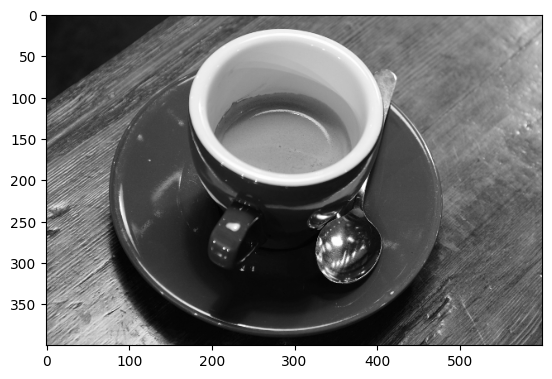
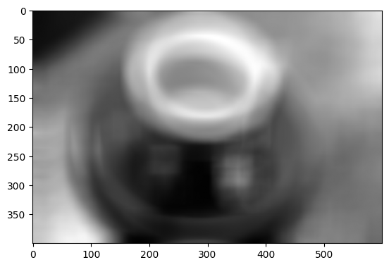
We’ll apply it to a grayscale coffee image, originally a color image from ski.data:
coffee_gray = ski.color.rgb2gray(ski.data.coffee())
plt.imshow(coffee_gray);
But first, we will use Numpy to add some normally distributed (Gaussian) noise to the image:
# Add some noise to the pixel values in `coffee`.
rng = np.random.default_rng()
# Mean 0, std 2 normal random numbers.
noisy_coffee_gray = coffee_gray + rng.normal(0, 2, size=coffee_gray.shape)
plt.imshow(noisy_coffee_gray);
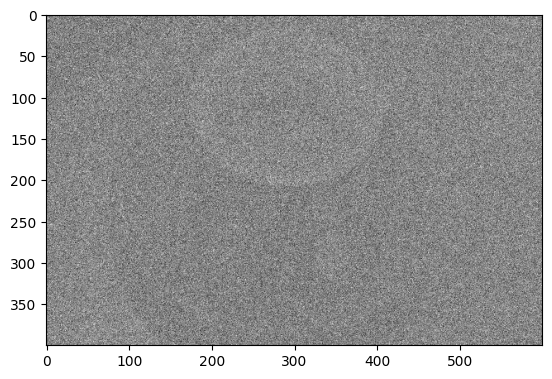
The mean filter can remove some of the noise, restoring the clarity of the image. This works because the noise varies randomly around 0 from pixel to pixel. Taking an average of random numbers with mean 0 (as here) will, on average, give a number closer to 0 than the original random numbers. However, the underlying (noise-free) image has some consistency from pixel to pixel, caused by the features of the image — such as the cup, in this case. Although the averaging leads to blurring of the underlying image, it doesn’t suppress it to anything like the same extent as the pixel-to-pixel noise.
# Mean filter the noisy coffee image, and show the result.
noisy_coffee_gray_mean_filtered = mean_filter(noisy_coffee_gray, (10, 10))
plt.figure(figsize=(20, 20))
plt.subplot(1, 3, 1)
plt.imshow(coffee_gray)
plt.title("Original")
plt.axis('off')
plt.subplot(1, 3, 2)
plt.title('Noisy')
plt.imshow(noisy_coffee_gray)
plt.axis('off')
plt.subplot(1, 3, 3)
plt.title('Mean Filtered')
plt.imshow(noisy_coffee_gray_mean_filtered)
plt.axis('off');
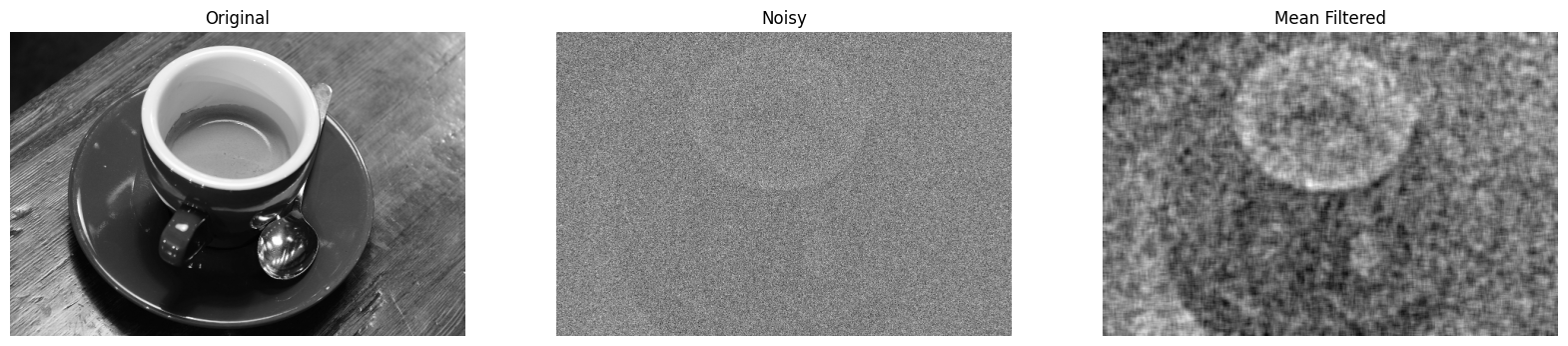
We can see that the image is clearer, the noise has been reduced and some of the signal has been restored.
Let’s try out some different kernel sizes:
# Mean filter, with various kernel sizes.
n_cols = 3
plt.figure(figsize=(12, 7))
plt.subplot(2, n_cols, 1)
plt.imshow(coffee_gray)
plt.title("Original")
plt.axis('off')
plt.subplot(2, n_cols, 2)
plt.title('Noisy')
plt.imshow(noisy_coffee_gray)
plt.axis('off')
for i in range(3, int(n_cols*2)+1):
    plt.subplot(2, n_cols, i)
    kernel_shape = (i+(i*3), i+(i*3))
    plt.title(f'Mean Filtered\nKernel = ({i+(i*3)},{i+(i*3)})')
    plt.imshow(mean_filter(noisy_coffee_gray, kernel_shape))
    plt.axis('off')
plt.subplots_adjust()
plt.tight_layout();
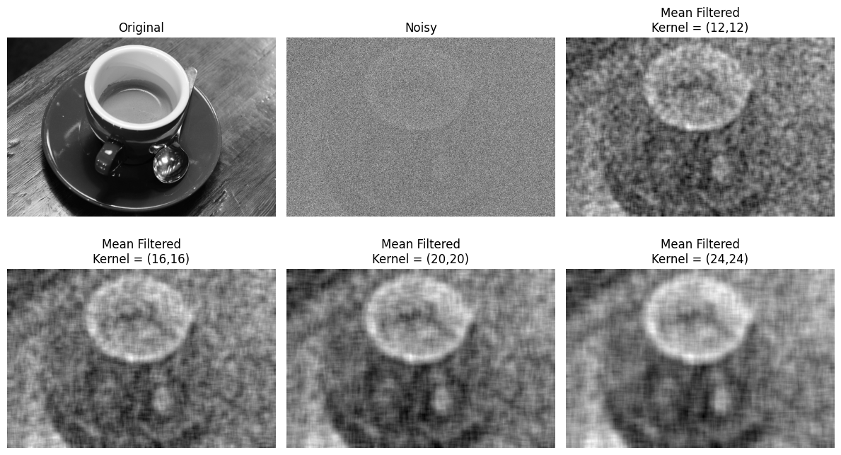
As with many filtering operations, the effect of altering aspects of the filtering process (like a threshold value or kernel size), is very context-dependent. It may take many iterations before finding a “sweet spot”, and where the sweet spot is may be somewhat subjective.
Exercise 22
The nice thing about applying filtering via kernels is that changing the kernel
itself lets us implement a wide variety of functions, even fairly strange ones.
In this exercise, you will write a function called strange_filter(). You
should apply it to coffee_gray to produce the following image:
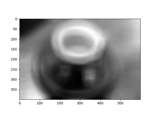
The kernel we used, and that we want you to us, was one where the kernel value was proportional to the Euclidean distance from the kernel center. That is, if \(i\) is the first (row) index of the kernel, and j is the second (column) index of the kernel, the kernel value at coordinate \(i, j\) is given by:
where \(c_i\) and \(c_j\) are the coordinates of the center pixel in the kernel.
Notice this gives higher weight to pixels that are further from the center.
You might remember this kind of idea from the circular mask in the mask section. Look there for inspiration.
Write your function so that it can be used with kernels of different shapes, so you can work out what kernel shape you need to recreate the target image, by trial and error.
DO NOT COPY THE mean_filter() FUNCTION FROM ABOVE AND MODIFY IT - try to write a function from scratch, thinking carefully about what you need to do.
Hint: You will need a fairly large kernel to get the effect you want.
Hint: run the hint.strange_coffee() function for additional help.
# YOUR CODE HERE
strange_coffee = coffee_gray.copy()

# Show `strange_coffee`.
plt.imshow(strange_coffee)
show_attributes(strange_coffee)
Type: <class 'numpy.ndarray'>
dtype: float64
Shape: (400, 600)
Max Pixel Value: 1.0
Min Pixel Value: 0.0
Solution to Exercise 22
The solution here involves adapting the code you find in the mask section, to build the kernel. Let’s start by building a function to build the kernel for given kernel shape:
def euclid_kernel(kernel_shape):
# i and j coordinates in the kernel.
i_coords, j_coords = np.meshgrid(np.arange(kernel_shape[0]),
np.arange(kernel_shape[1]),
indexing='ij')
# Calculate distance for each pixel in kernel.
c_i, c_j = (np.array(kernel_shape) - 1) / 2
return np.sqrt((i_coords - c_i) ** 2 + (j_coords - c_j) ** 2)
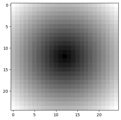
# Show a 25 by 25 kernel.
plt.imshow(euclid_kernel((25, 25)))
<matplotlib.image.AxesImage at 0x7ffb529691d0>
We define our strange_filter() function in the cell below:
def strange_filter_solution(image_array, kernel_shape):
    return ndi.correlate(image_array,
                         euclid_kernel(kernel_shape),
                         mode='reflect',  # The default.
                        )
To get the exact target image, we use a kernel of shape (50, 50):
# Apply the filter and show the result.
strange_filter_coffee = strange_filter_solution(coffee_gray, (50, 50))
show_attributes(strange_filter_coffee)
plt.imshow(strange_filter_coffee);
Type: <class 'numpy.ndarray'>
dtype: float64
Shape: (400, 600)
Max Pixel Value: 37834.72
Min Pixel Value: 1720.34
For reflection — why does the filtered image look as it does? See if you can explain its features, compared to the original.
This is quite a strange kernel to apply! But it shows us how easy it is to achieve radical filtering effects with some custom kernels…
Filtering 3D images#
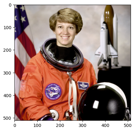
We can filter a 3D color image by applying our filtering kernel to each color channel separately. Let’s load a 3D image:
# Load in and show an image.
astronaut = ski.data.astronaut()
show_attributes(astronaut)
plt.imshow(astronaut);
Type: <class 'numpy.ndarray'>
dtype: uint8
Shape: (512, 512, 3)
Max Pixel Value: 255
Min Pixel Value: 0
If we try to filter this image with our (3, 3) mean_kernel we will get an error:
# Oh dear.
astronaut_mean_filtered = ndi.correlate(astronaut, weights=mean_kernel)
---------------------------------------------------------------------------
RuntimeError                              Traceback (most recent call last)
Cell In[39], line 2
      1 # Oh dear.
----> 2 astronaut_mean_filtered = ndi.correlate(astronaut, weights=mean_kernel)

File /opt/hostedtoolcache/Python/3.13.11/x64/lib/python3.13/site-packages/scipy/ndimage/_filters.py:1375, in correlate(input, weights, output, mode, cval, origin, axes)
   1309 @_ni_docstrings.docfiller
   1310 def correlate(input, weights, output=None, mode='reflect', cval=0.0,
   1311               origin=0, *, axes=None):
   1312     """
   1313     Multidimensional correlation.
   1314
   (...)   1373
   1374     """
-> 1375     return _correlate_or_convolve(input, weights, output, mode, cval,
   1376                                   origin, False, axes)

File /opt/hostedtoolcache/Python/3.13.11/x64/lib/python3.13/site-packages/scipy/ndimage/_filters.py:1277, in _correlate_or_convolve(input, weights, output, mode, cval, origin, convolution, axes)
   1275 wshape = [ii for ii in weights.shape if ii > 0]
   1276 if len(wshape) != input.ndim:
-> 1277     raise RuntimeError(f"weights.ndim ({len(wshape)}) must match "
   1278                        f"len(axes) ({len(axes)})")
   1279 if convolution:
   1280     weights = weights[tuple([slice(None, None, -1)] * weights.ndim)]

RuntimeError: weights.ndim (2) must match len(axes) (3)
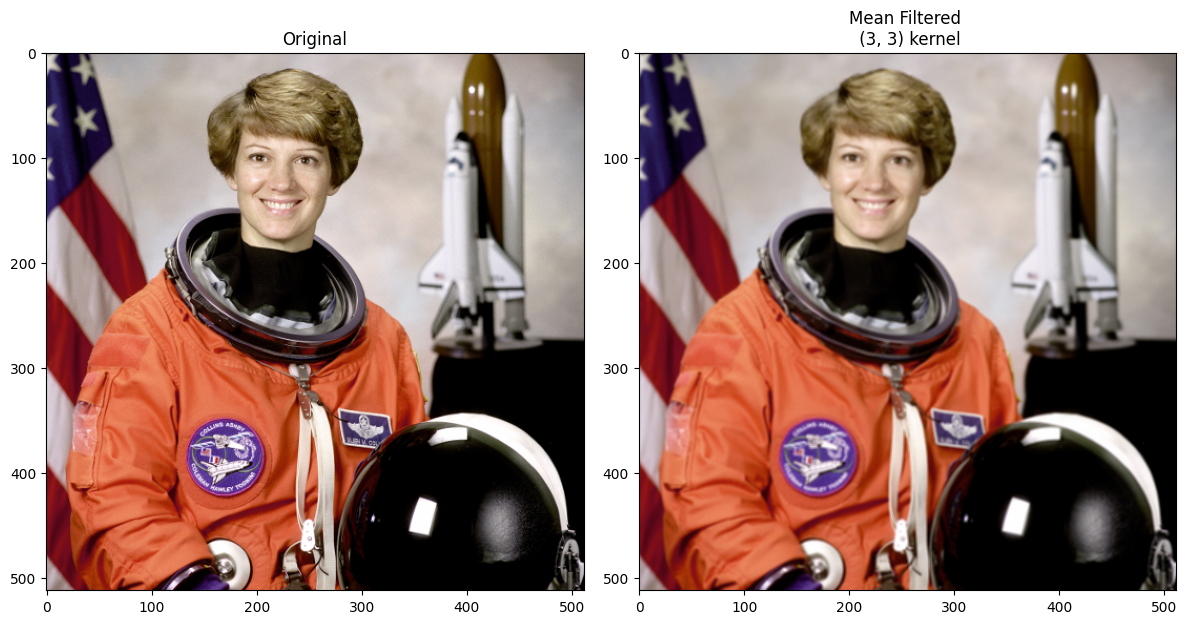
As you can see, the error results from using a 2D kernel to filter a 3D image. A simple solution to this is just to apply the filter to each color channel separately. This is done in the cell below, using a for loop to filter each channel, storing the channels separately in a dictionary, and then np.stack()-ing the individually filtered channels back into a 3D image:
# A dictionary to store the individually filtered channels.
filtered_channels = {}

# Loop through and filter each channel individually, store
# the results in the dictionary.
for i in range(astronaut.shape[2]):
    current_filtered_channel = ndi.correlate(astronaut[:, :, i],
                                             weights=mean_kernel)
    filtered_channels[i] = current_filtered_channel

# Stack back to 3D.
astronaut_mean_filtered = np.stack([filtered_channels[0],
                                    filtered_channels[1],
                                    filtered_channels[2]],
                                   axis=2)

# Show the result.
plt.figure(figsize=(12, 6))
plt.subplot(1,2,1)
plt.title("Original")
plt.imshow(astronaut)
plt.subplot(1,2,2)
plt.title("Mean Filtered \n (3, 3) kernel")
plt.imshow(astronaut_mean_filtered)
plt.tight_layout();
This is straightforward to do with skimage as well; we also use the larger
(9, 9) footprint_9_by_9 kernel:
# A dictionary to store the individually filtered channels.
filtered_channels = {}

# Loop through and filter each channel individually, store
# the results in the dictionary.
for i in range(astronaut.shape[2]):
    current_filtered_channel = ski.filters.rank.mean(  # skimage filtering.
        astronaut[:, :, i],
        footprint=footprint_9_by_9) # Use a larger kernel.
    filtered_channels[i] = current_filtered_channel

# Stack back to 3D.
astronaut_mean_filtered = np.stack([filtered_channels[0],
                                    filtered_channels[1],
                                    filtered_channels[2]],
                                   axis=2)

# Show the result.
plt.figure(figsize=(12, 6))
plt.subplot(1,2,1)
plt.title("Original")
plt.imshow(astronaut)
plt.subplot(1,2,2)
plt.title("Mean Filtered with `ski.filters.rank.mean()` \n (9, 9) kernel")
plt.imshow(astronaut_mean_filtered)
plt.tight_layout();
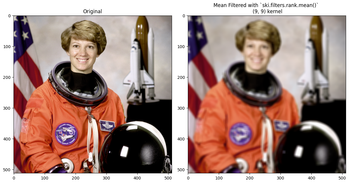
We got a blurrier output image via skimage here, than in the kernel filter
using ndi.correlate(). This is because we used a larger kernel for the
skimage filtering, and so are averaging over larger pixel neighborhoods.
Scikit-image will also handle this using a 3D kernel.
footprint_9_by_9_3D = np.ones((9, 9, 3))
# Mean filter the color image, with `skimage`.
astronaut_mean_filtered_ski = ski.filters.rank.mean(astronaut,
                                                    footprint=footprint_9_by_9_3D)

# Show the result.
plt.figure(figsize=(12, 6))
plt.subplot(1,2,1)
plt.title("Original")
plt.imshow(astronaut)
plt.subplot(1,2,2)
plt.title("Mean Filtered (via Scikit-image)\n (9, 9) kernel")
plt.imshow(astronaut_mean_filtered_ski)
plt.tight_layout();
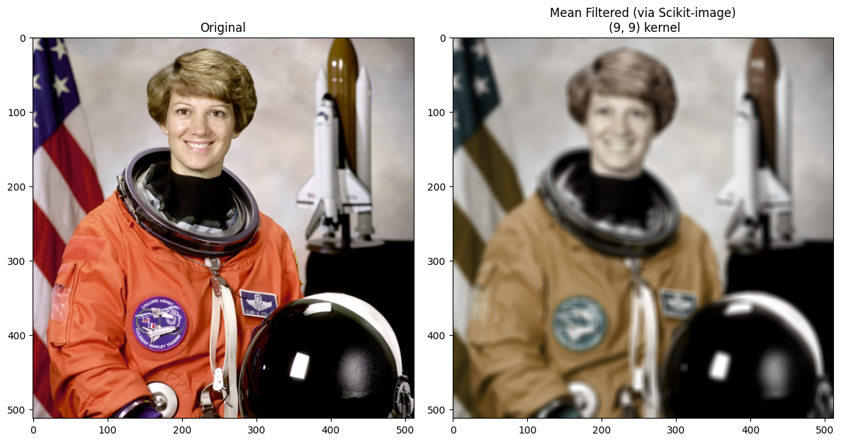
Pay attention here to the effect on the color of the image. How is it different to filtering the color channels separately?
You’ll notice that the colors have changed substantially, relative to when we filtered each channel separately. This is because the 3D kernel is averaging across the color channels. We may want this effect (it is somewhat retro), but if we do not want to mix the color channels of the image, then generally filtering the channels separately is the way to go…
Summary#
This page has showed how to perform mean filtering, using numpy, scipy and
skimage. On the next page, we will look at
using different kernels to get different filtering effects.
References#
Gulati, J. (2024) NumPy for Image Processing. KDnuggets. Available from: https://www.kdnuggets.com/numpy-for-image-processing
Adapted from: