More filters: the median filter and non-local filters

Note

This tutorial is adapted from “Image manipulation and processing using NumPy and SciPy” by Emmanuelle Gouillart and Gaël Varoquaux, and “scikit-image: image processing” by Emmanuelle Gouillart. Please see the References section at the end of the page for other sources and resources.

This page will cover filters which do not use filtering kernels. First, we will look at the median filter, which differs in important ways from the other local filters we saw on previous pages, because it cannot be implemented through kernels. In fact, it is a footprint/function filter.

After the median filter, we will look at another filter, the histogram equalisation filter, which does not use kernel methods. In fact, histogram equalisation does not use a footprint at all. Because it eschews footprints completely, the histogram equalisation filter is a non-local filter. More on this below.

As normal, we begin with some imports:

# Library imports.
import numpy as np
import matplotlib.pyplot as plt
import skimage as ski

# Set 'gray' as the default colormap
plt.rcParams['image.cmap'] = 'gray'

# Set NumPy precision to 2 decimal places
np.set_printoptions(precision=2)

# A custom function to quickly report image attributes.
from skitut import show_attributes

Local filtering without kernels

When compared to the other local filters we have seen, the median filter uses the same process of “walking” through the image with a small footprint array that defines the “local neighborhood” of each pixel.

Median filtering is an example of footprint/function filtering. That is, the footprint defines the local neighborhood, and we apply the np.median function to that local neighborhood.

Note

Footprints and kernels

Remember — a footprint is a binary (True / False, 1 / 0) array defining the pixel neighborhood. A kernel is a footprint with weights.

As with the other footprints and kernels we have seen, the footprint is centered on every pixel during the filtering operation. The central pixel value is replaced with a number computed from the other values in the local neighborhood, e.g. the other pixel values under the footprint.

When we apply a kernel, we calculate the new pixel value by taking a weighted sum of the pixels in the neighborhood, defined by the weights in the kernel.

Footprint / function filters, such as the median filter, work in a different way. They first select the pixels within the neighborhood, using the footprint, and then apply a function to the selected (neighborhood) pixel values. The median filter, you will not be astonished to hear, takes the median value of the pixels under the footprint.

There is no way of using a kernel (a weighted sum) to calculate the median, and this is why we and others will remind to be careful to distinguish footprint filters (and footprints) from kernel filters (and kernels).Calculating the median utilizes ranking and indexing, and cannot be expressed as a weighted sum, in the way that calculating a mean can, for instance.

One way to think of this, is that when we write the formula for the mean, we can write it without reference to any Python indexing operations:

\( \large \text{mean} = \frac{\sum X}{n} \)

…we can read that as “to get the mean of a set of numbers (where \(X\) refers all of the numbers), add them up and divide by however many numbers there are (\(n\))”.

Conversely for the median we first have to order the numbers from lowest to highest (\(X_{\text{sorted}}\)), and then find the value that is at the central index. So where \(X\) is an array containing all the numbers, if \(n\) is odd:

\( \large \text{median} = X_{\text{sorted}}[\frac{n - 1}{2}]\)

— where the square brackets are an indexing operation.

Recall that, in Python, indices start at 0, and therefore, the central element is at index \(\frac{n - 1}{2}\).

Consider the numbers in the array below:

# Some numbers.
nums = np.array([10, 4, 5, 8, 7])
nums

array([10,  4,  5,  8,  7])

We get the mean from: \( \large \text{mean} = \frac{\sum x_i...x_n}{n} \)

# Take the sum, divide by n.
np.sum(nums) / len(nums)

np.float64(6.8)

# Compare to the same calculation from NumPy.
np.mean(nums)

np.float64(6.8)

Whereas we get the median from: \( \large \text{median} = X_{\text{sorted}}[\frac{n - 1}{2}]\)

# Get the median.
sorted_nums = np.sort(nums) # Sort the values, low to high.
print(f"Sorted `nums`: {sorted_nums}")
median = sorted_nums[int(len(sorted_nums)/2)] # Index to get the median.

# Show the median value.
median

Sorted `nums`: [ 4  5  7  8 10]

np.int64(7)

# Compare to NumPy.
np.median(nums)

np.float64(7.0)

Note

Median and even-length arrays

You will have spotted at once that the central position \(\frac{n - 1}{2}\) will not be an integer for even-length arrays. In code, the central position is c = (len(arr) - 1) / 2, and, for even-length arrays (len(arr) is even), c will not be an integer.

np.median solves this in the standard way, by giving the median value as the mean of the values in the sorted array at indices np.floor(c) and np.ceil(c) — in other words, the mean of the sorted values either side of position c.

There is no kernel method that can do the median calculation, because the median cannot be expressed as a weighted sum. Instead we use the footprint to define a pixel neighborhood, then replace the central value with the median from that neighborhood, using the sorting and indexing we have seen above. So, the median filter is a local filter, because it alters pixel values based on other pixel values in the local neighborhood (footprint). However, it is not a kernel filter because it does not use a weighted sum of the local neighborhood, in contrast to other kernel-based filters like the mean filter, Gaussian filter etc.

Edge preservation

The median filter is especially useful for removing noise from images, while preserving the “edges” in the image. You’ll recall that the edges are big changes in the gradient of pixel intensities, between nearby pixels (e.g. black-to-white, white-to-black etc). Let’s look at why the median filter is “edge preserving”, by expanding the nums array into a low-resolution image, using np.tile() and np.reshape().

# Make `nums` into a image array.
nums_img = np.reshape(np.tile(nums, reps=3), (3, 5))
nums_img

array([[10,  4,  5,  8,  7],
       [10,  4,  5,  8,  7],
       [10,  4,  5,  8,  7]])

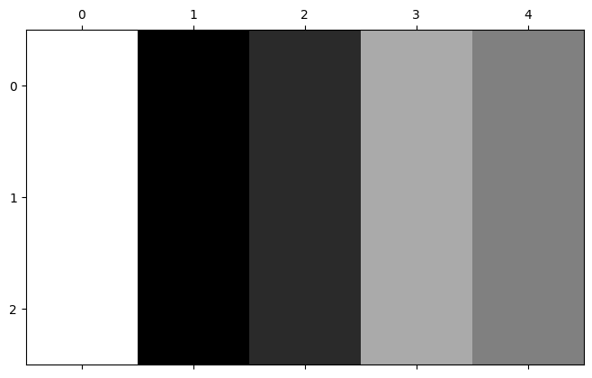
# Show as an image.
plt.matshow(nums_img);

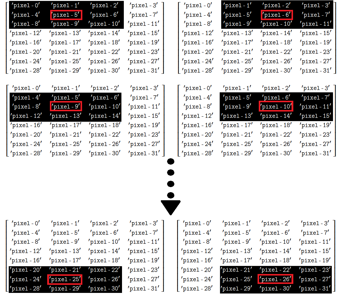
Now, imagine we “walk” a 3-by-3 footprint through the nums_img array, and replace the central pixel of each footprint with the median of the pixels under the kernel.

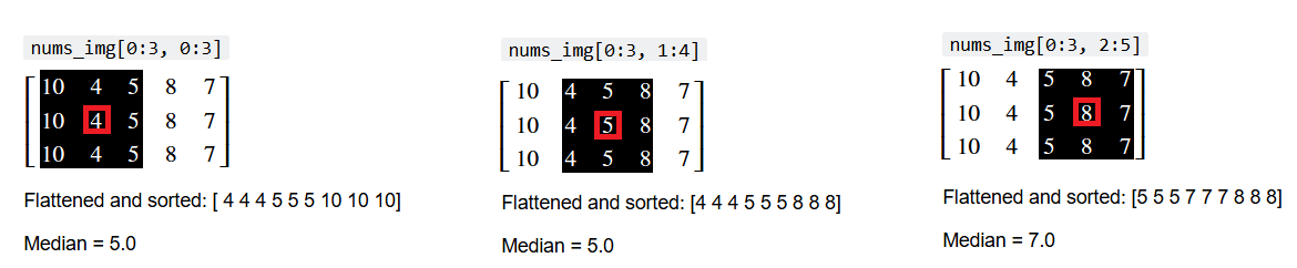
This process is shown below, for three footprints (“local neighborhoods” under a 3-by-3 array). The central pixel is highlighted in red, and the index of the current local neighborhood is shown above the pixel values.

The flattened and sorted values from each local neighborhood are also shown, along with the median value of the neighborhood:

We can also show this in “Python space”, using a for loop:

# Show some local neighborhoods of `nums_img` and their medians.
for i in range(3):
    i_row_start, i_col_start = 0, i
    i_row_end, i_col_end = 3, i + 3
    print(f"\nnums_img[{i_row_start}:{i_row_end}, {i_col_start}:{i_col_end}]")
    current_selection = nums_img[i_row_start:i_row_end, i_col_start:i_col_end]
    print(current_selection)
    print(f"Flattened and sorted: {np.sort(current_selection.ravel())}")
    print(f"Median = {np.median(nums_img[i_row_start:i_row_end, i_col_start:i_col_end])}")

nums_img[0:3, 0:3]
[[10  4  5]
 [10  4  5]
 [10  4  5]]
Flattened and sorted: [ 4  4  4  5  5  5 10 10 10]
Median = 5.0

nums_img[0:3, 1:4]
[[4 5 8]
 [4 5 8]
 [4 5 8]]
Flattened and sorted: [4 4 4 5 5 5 8 8 8]
Median = 5.0

nums_img[0:3, 2:5]
[[5 8 7]
 [5 8 7]
 [5 8 7]]
Flattened and sorted: [5 5 5 7 7 7 8 8 8]
Median = 7.0

Because the median is not a function that can be applied via kernel filtering, we cannot apply it using ndi.correlate(), as we did with the other local filters.

We can apply the median filter in skimage using ski.filters.median(). Again, we supply a footprint argument to determine the size and shape of each pixel’s “local neighborhood”:

# Median filter `nums_img`.
nums_median_filtered = ski.filters.median(nums_img,
                                          footprint=np.ones((3,3)))
nums_median_filtered

array([[10,  5,  5,  7,  7],
       [10,  5,  5,  7,  7],
       [10,  5,  5,  7,  7]])

Compare to the original nums_img array below:

nums_img

array([[10,  4,  5,  8,  7],
       [10,  4,  5,  8,  7],
       [10,  4,  5,  8,  7]])

The effect on the “edges” of the image is easier to see graphically:

# Show the images.
plt.subplot(1, 2, 1)
plt.imshow(nums_img)
plt.title('Original')
plt.subplot(1, 2, 2)
plt.imshow(nums_median_filtered)
plt.title('Median Filtered');

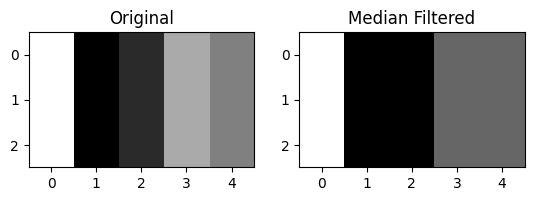
Edges involving a bigger gradient have been preserved, whilst less prominent edges have been merged into more prominent ones nearby. We show this, for comparison, alongside a mean filtered version of nums_img, filtered using the same size footprint ((3, 3)):

# Avoid dtype warning.  In our case, `nums_img` already fits within the 
# np.uint8 range (0 to 255).
nums_img = nums_img.astype(np.uint8)
nums_mean_filtered = ski.filters.rank.mean(nums_img,
                                           footprint=np.ones((3,3)))
# Show the images.
plt.figure(figsize=(12, 4))
plt.subplot(1, 3, 1)
plt.imshow(nums_img)
plt.title('Original')
plt.subplot(1, 3, 2)
plt.imshow(nums_median_filtered)
plt.title('Median Filtered')
plt.subplot(1, 3, 3)
plt.imshow(nums_mean_filtered)
plt.title('Mean Filtered');

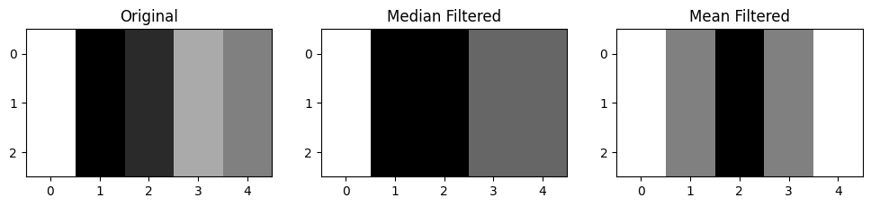
You can see that the median filter gives a better “summary” of the distribution of edges in the original image - the mean filter has blurred the edges more, which makes sense, given that it averages pixels within a kernel.

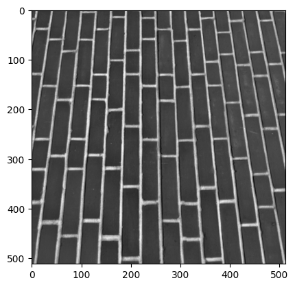
In a higher resolution image, the median filter can have the effect of removing noise whilst preserving edges to a greater extent than some other filters. We will demonstrate the median filter again with the brick image from ski.data:

# Load in the `brick` image.
brick = ski.data.brick()
show_attributes(brick)
plt.imshow(brick);

Type: <class 'numpy.ndarray'>
dtype: uint8
Shape: (512, 512)
Max Pixel Value: 207
Min Pixel Value: 63

We will also filter brick using a mean filter, with the same size kernel as the median filter:

# Apply a median filter.
median_filtered_brick = ski.filters.median(brick,
                                           footprint=np.ones((9,9)))

mean_filtered_brick = ski.filters.rank.mean(brick,
                                            footprint=np.ones((9,9)))
# Plot both image to compare
plt.figure(figsize=(14, 4))
plt.subplot(1, 3, 1)
plt.title('Original Image')
plt.imshow(brick)
plt.subplot(1, 3, 2)
plt.title('Median Filtered')
plt.imshow(median_filtered_brick)
plt.subplot(1, 3, 3)
plt.title('Mean Filtered')
plt.imshow(mean_filtered_brick);

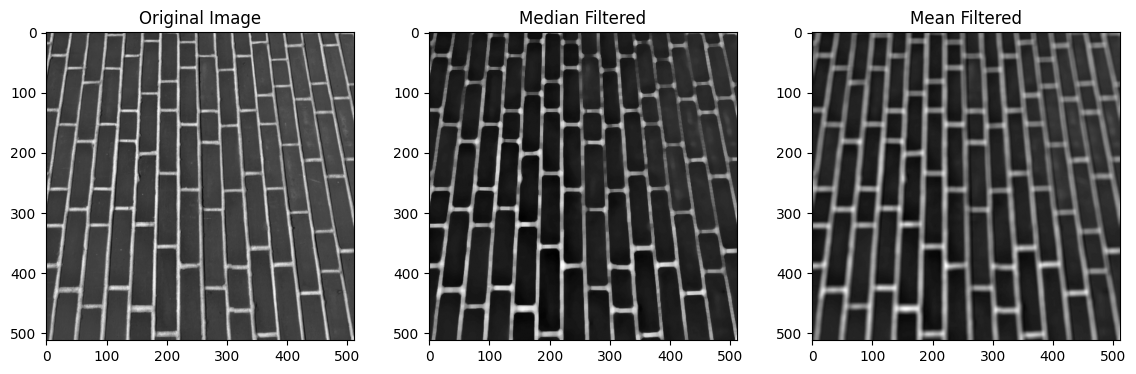
You can see that the edges in the images (transitions between pixels of very different intensities - in this case between the dark bricks and the lighter mortar lines) are less smoothed (less blurred) by the median filter than by the mean filter. This can be a desirable property of the median filter, depending on your application.

Non-local filters

Whilst the median filter does not use a kernel, it is still a local filter, because it filters pixels based on the values of other pixels in the local neighborhood, defined by footprint. Other filters use neither kernel filtering nor a local pixel neighborhood. These filters are called non-local filters.

Non-local filters filter all of pixels in an image based on characteristics of a specific region of the image, or based upon characteristics of the entire image. As a result, a non-local filter might modify a given pixel’s value based on the values of pixels in parts of the image that are nowhere near the “local neighborhood” of the pixel being modified.

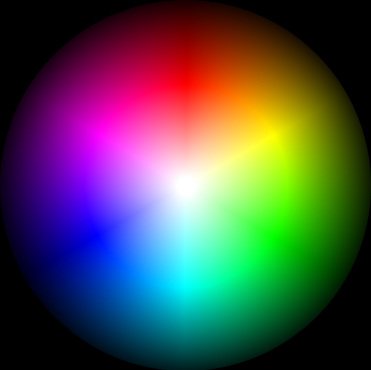
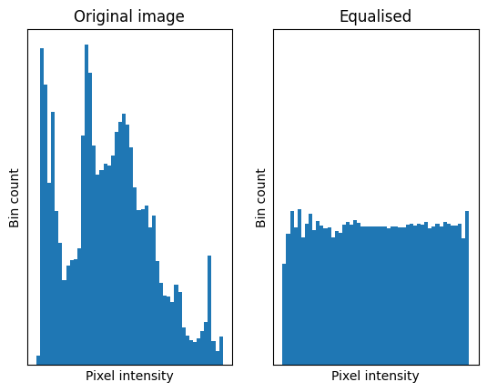
One foundational non-local filter is a histogram equalisation filter. This filter modifies pixels based on the intensity histogram of the entire image. Essentially, this process flattens the image intensity histogram into a uniform distribution, so that there is less variance between the pixel intensities. The image below illustrates this principle:

Show code cell source

Hide code cell source

gray_coffee = ski.color.rgb2gray(ski.data.coffee())
eq_coffee = ski.exposure.equalize_hist(gray_coffee)
plt.subplot(1, 2, 1)
edges, counts, obj = plt.hist(gray_coffee.ravel(), bins=50);
ylims = plt.ylim()
plt.xticks([])
plt.yticks([])
plt.xlabel('Pixel intensity')
plt.ylabel('Bin count')
plt.title('Original image')
plt.subplot(1, 2, 2)
plt.hist(eq_coffee.ravel(), bins=50)
plt.ylim(ylims)
plt.xticks([])
plt.yticks([])
plt.xlabel('Pixel intensity')
plt.ylabel('Bin count')
plt.title('Equalised');

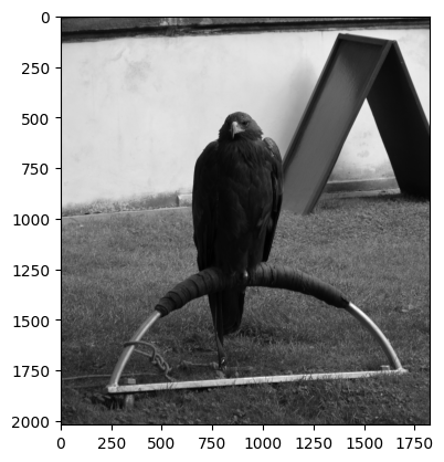
We will demonstrate the histogram equalisation filter with the eagle image from ski.data:

# Load in the `eagle` image.
eagle = ski.data.eagle()
show_attributes(eagle)
plt.imshow(eagle);

Type: <class 'numpy.ndarray'>
dtype: uint8
Shape: (2019, 1826)
Max Pixel Value: 255
Min Pixel Value: 1

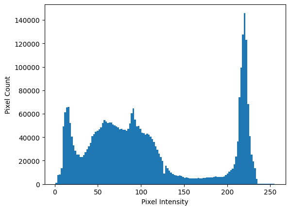
Let’s first view the intensity histogram of eagle, before we apply the filter. As we know, we can use the .ravel() array method to flatten this 2D image to 1D, and then inspect a histogram of the pixel intensities:

# Flatted to 1D.
one_D_eagle = eagle.ravel()

# Show a histogram.
plt.hist(eagle.ravel(),
         bins=128)
plt.xlabel('Pixel Intensity')
plt.ylabel('Pixel Count');

In order to apply the histogram equalisation filter, we first “deconstruct” into separate arrays using np.histogram(). This returns two arrays. One array we will call counts; this contains the height of the histogram within each \(x\)-axis bin. The second array we will call bin_intervals; adjacent values in this array are the start and end points of each \(x\)-axis bin. We use bin_intervals to calculate the center point of each bin, by taking the average of the adjacent values.

Note: we could also use ski.exposure.histogram(), to the same effect.

# Centers and bin intervals, from the histogram of the flattened `eagle` image.
counts, bin_intervals = np.histogram(one_D_eagle,
                                     bins=256)

# Calculate the bin centers from the bin edges.
bin_centers = (bin_intervals[1:] + bin_intervals[:-1]) / 2

# Show the `counts` and `bin_centers`.
print(f"\nCounts:\n {counts}")
print(f"\nBin centers:\n {bin_centers}")

Counts:
 [   15  1043  3803  3794  3947  4188  4896  8568 20430 28813 31334 30073
 32479 32788 34573 31031 27093 24958 21171 19158 17292 15934 14911 13743
 12428 12894 13134 12139 11564 11392 11656 11526 12260 12662 12633 14518
 14749 15056 16000 16111 17366 17689 20367 20406 20800 21776 22269 22562
 22734 22867 22502 24081 23931 24568 25676 26440 27242 27198 26991 26576
 26036 25940 26447 26010 26785 25571 25465 25381 25014 24989 24750 24288
 24369 24221 23456 23455 23117 23846 22988 23418 23675 22659 22424 22875
 22995 23989 24890 26900 28706 31551 32768 31771 28655 26372 24775 24297
 25018 24581 24102 22856 22137 21587 21997 21338 21149 21068 21519 21369
 21180 20819 20446 20098 19616 18770 18186 17627 16392 15842 15282 14066
 13442 12730 11799 11113 10171  9469  8993     0  8181  7597  7045  6393
  5980  5540  5258  4733  4464  4244  3997  3763  3688  3636  3547  3470
  3626  3761  3510  3373  3191  2843  2578  2689  2670  2873  2673  2549
  2484  2574  2493  2375  2336  2502  2325  2386  2454  2420  2555  2662
  2447  2357  2443  2458  2607  2603  2585  2754  2852  2855  2884  2932
  2804  2752  2727  2779  2881  3043  3138  3194  3137  2972  2952  2981
  3020  3070  3056  3107  3232  3456  3746  3869  4302  4607  4938  5891
  5986  6004  6359  6820  7832  9182 10684 12756 15987 20194 30541 43369
 48839 50582 58332 69319 72665 73282 66447 56525 39541 28719 22021 18822
 13779 11236  9769  9417  7775  5592  3467  1043   222   146   116    94
   113   109    90   119   104   105   126   109    94   122    94    95
    88   339   244     2]

Bin centers:
 [  1.5    2.49   3.48   4.47   5.46   6.46   7.45   8.44   9.43  10.43
  11.42  12.41  13.4   14.39  15.39  16.38  17.37  18.36  19.36  20.35
  21.34  22.33  23.32  24.32  25.31  26.3   27.29  28.29  29.28  30.27
  31.26  32.25  33.25  34.24  35.23  36.22  37.21  38.21  39.2   40.19
  41.18  42.18  43.17  44.16  45.15  46.14  47.14  48.13  49.12  50.11
  51.11  52.1   53.09  54.08  55.07  56.07  57.06  58.05  59.04  60.04
  61.03  62.02  63.01  64.    65.    65.99  66.98  67.97  68.96  69.96
  70.95  71.94  72.93  73.93  74.92  75.91  76.9   77.89  78.89  79.88
  80.87  81.86  82.86  83.85  84.84  85.83  86.82  87.82  88.81  89.8
  90.79  91.79  92.78  93.77  94.76  95.75  96.75  97.74  98.73  99.72
 100.71 101.71 102.7  103.69 104.68 105.68 106.67 107.66 108.65 109.64
 110.64 111.63 112.62 113.61 114.61 115.6  116.59 117.58 118.57 119.57
 120.56 121.55 122.54 123.54 124.53 125.52 126.51 127.5  128.5  129.49
 130.48 131.47 132.46 133.46 134.45 135.44 136.43 137.43 138.42 139.41
 140.4  141.39 142.39 143.38 144.37 145.36 146.36 147.35 148.34 149.33
 150.32 151.32 152.31 153.3  154.29 155.29 156.28 157.27 158.26 159.25
 160.25 161.24 162.23 163.22 164.21 165.21 166.2  167.19 168.18 169.18
 170.17 171.16 172.15 173.14 174.14 175.13 176.12 177.11 178.11 179.1
 180.09 181.08 182.07 183.07 184.06 185.05 186.04 187.04 188.03 189.02
 190.01 191.   192.   192.99 193.98 194.97 195.96 196.96 197.95 198.94
 199.93 200.93 201.92 202.91 203.9  204.89 205.89 206.88 207.87 208.86
 209.86 210.85 211.84 212.83 213.82 214.82 215.81 216.8  217.79 218.79
 219.78 220.77 221.76 222.75 223.75 224.74 225.73 226.72 227.71 228.71
 229.7  230.69 231.68 232.68 233.67 234.66 235.65 236.64 237.64 238.63
 239.62 240.61 241.61 242.6  243.59 244.58 245.57 246.57 247.56 248.55
 249.54 250.54 251.53 252.52 253.51 254.5 ]

We chose to use 256 bins, for this histogram, for reasons that will become apparent further down the page (remember this!).

There are several steps in equalising the histogram:

1. We normalise the histogram, so that the counts sum to 1. We do this by dividing each count by the total number of pixels in the image, which converts each count to a proportion.

2. Then we calculate the cumulative density of the normalised histogram. Basically, this means we add up the proportions as we go along the \(x\)-axis, so each bin indicates the total proportion of pixels up to that point (ie pixels in that particular bin, or bins situated lower down the \(x\)-axis).

3. We “map” each pixel intensity value to its corresponding cumulative proportion. After this “mapping”, we have our equalised histogram.

This may all sound quite abstract, but bear with us. It is easier to follow in code, and is a visually striking effect when we compare the resulting histogram to the original.

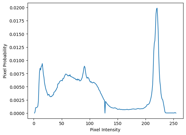
For the first step, we can normalise the counts by dividing each individual count by the total number of pixels in the image. Note that we could also do this using the optional density=True argument to np.histogram(), but we do it manually to show what the operations involve:

# Centers and bin intervals, from the histogram of the flattened `eagle` image.
# Get the total number of pixels.
n_pixels = len(one_D_eagle)
# Normalize by dividing each count by the total number of pixels.
counts_normed = counts/n_pixels
plt.plot(bin_centers, counts_normed)
plt.xlabel('Pixel Intensity')
plt.ylabel('Pixel Probability');

# Do the `counts` sum to 1?
print(f"\nCounts Normalized sum:\n {counts_normed.sum()}")

Counts Normalized sum:
 1.0

When we equalise the histogram, we want it to be roughly uniform across the pixel intensities. As a tool to perform this “uniformization”, we first we calculate the cumulative distribution (cdf) of the histogram. To do this we take cumulative sum of the normalised counts (counts_normed). For a given bin, the cumulative sum operation adds up the proportion of pixels that are in that bin and in all of the lower bins (e.g. the bins closer to 0 on the \(x\)-axis). Essentially it is a running total of the counts_normed as we move from left to right across the \(x\)-axis:

# Get the cumulative distribution of the pixel intensities.
cdf = np.cumsum(counts_normed)

# Show a plot of the cumulative distribution.
plt.plot(bin_centers, cdf)
plt.xlabel('Pixel Intensity')
plt.ylabel('Cumulative Proportion');

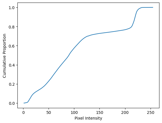
The final value in cdf is 1 (or at least close-as-dammit, given precision loss in the calculations). Remember, we are adding up proportions here, so a value of 1 indicates that the final bin and all of the lower bins together contain 100% (proportion 1.0) of the pixels in the image:

cdf[-1]

np.float64(0.9999999999999999)

The next step requires some thought, to follow what is going on. We want to “map” the pixel values in the flattened one_D_eagle array to the values in the cdf. We can do this, for the current eagle image, by using the one_D_eagle pixel intensity values as indexes for the cdf array. This might seem like a hack, so lets break it down.

Recall that we asked you to remember that we asked np.histogram() to give us a histogram with 256 bins? Well, as a result our cdf array, which contains the running total of the proportions in a given bin and lower bins, has 256 elements:

# Show the `shape` of the `cdf` array.
cdf.shape

(256,)

Because we count from 0, when indexing arrays, the final value in cdf is at index location 255:

# Show the final value of the `cdf` array, at integer index location 255.
cdf[255]

np.float64(0.9999999999999999)

Given that one_D_eagle is in the uint8 dtype, the maximum and minimum values allowed are 255 and 0. The actual image is has maximum, minimum of 255 and 1.

# Show the `dtype` and `min`/`max` values of `eagle`.
show_attributes(one_D_eagle)

Type: <class 'numpy.ndarray'>
dtype: uint8
Shape: (3686694,)
Max Pixel Value: 255
Min Pixel Value: 1

Conveniently here, each pixel intensity value in one_D_eagle will work as an index into cdf. This allows us to replace each pixel intensity value with its corresponding cumulative proportion. So, if a pixel intensity value \(p\) falls in bin \(b\), then bin \(b\) has a corresponding cumulative proportion in the cdf array. We use this “mapped” values as our output image - this has the effect of “smoothing out”, or, in fact, “equalising” the histogram, because bins without many pixels in them “inherit” the proportions from lower bins. Again, this is easier to appreciate visually, by viewing the histograms below.

Let’s perform the indexing/equalisation, and then inspect the histograms, so this effect becomes apparent. We show this mapping first with ten pixel intensity values from one_D_eagle:

first_ten_pixels = one_D_eagle[:10]
first_ten_pixels

array([18, 17, 17, 17, 16, 16, 17, 17, 16, 15], dtype=uint8)

…we then show the corresponding cumulative proportions that these values will be mapped to, when we use them as indexes for cdf:

cdf[first_ten_pixels]

array([0.09, 0.09, 0.09, 0.09, 0.08, 0.08, 0.09, 0.09, 0.08, 0.07])

To perform this mapping for every pixel intensity value, we use the following operation:

# Equalise the histogram of `eagle`, by using the pixel intensity values in `one_D_eagle` (1 - 255)
# as indexes into the `cdf` array.
equalised_hist = cdf[one_D_eagle]

The original histogram and the equalised histogram, along with the corresponding images, are shown below. We first .reshape() the equalised_hist back into the shape of the original, non-flattened eagle image, thus restoring its status as a 2D image array:

# Reshape to 2D.
eagleback_to_2D = equalised_hist.reshape(eagle.shape)

# Generate the plot.
plt.figure(figsize=(14, 8))
plt.subplot(2, 2, 1)
plt.imshow(eagle)
plt.title('Original Image')
plt.subplot(2, 2, 2)
plt.title('Original Histogram')
plt.hist(eagle.ravel(), bins=128)
plt.subplot(2, 2, 3)
plt.imshow(eagleback_to_2D)
plt.title('Equalised Image')
plt.subplot(2, 2, 4)
plt.title('Equalised Histogram')
plt.hist(eagleback_to_2D.ravel());

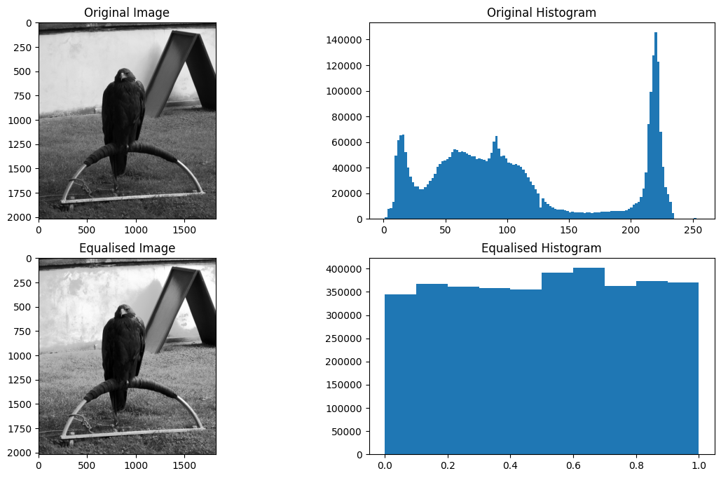
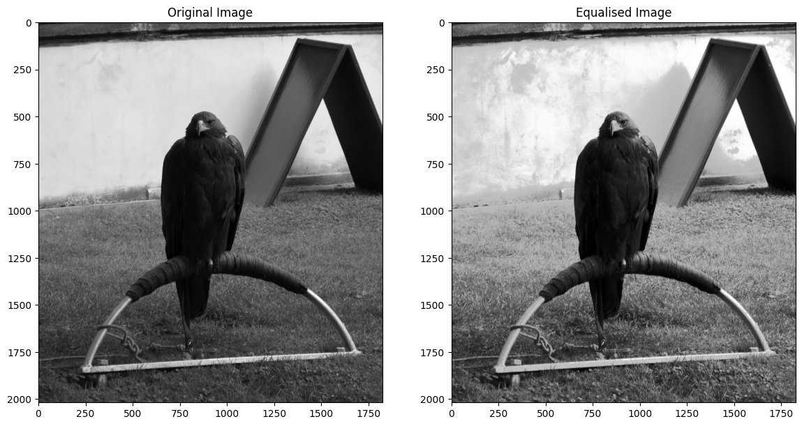
The equalised histogram now much more closely resembles a uniform distribution - the notable “peaks and valleys” of the original and been replaced with a uniform distribution. In this case, the effect on the perceived visual image is one of heightened contrast — pay particular attention to the wall behind the noble eagle. Each image, without the histograms, can be viewed below, for easier inspection:

# Generate the plot.
plt.figure(figsize=(14, 8))
plt.subplot(1, 2, 1)
plt.imshow(eagle)
plt.title('Original Image')
plt.subplot(1, 2, 2)
plt.imshow(eagleback_to_2D)
plt.title('Equalised Image');

Let’s consider how the equalisation works. Consider the original normalised (density) histogram and the cumulative density that we calculated above:

plat_x = [130, 200]
fig, ax = plt.subplots(2, 1)
ax[0].plot(bin_centers, counts_normed)
ax[0].set_ylabel('Intensity proportion');
ax[0].set_title('Proportional histogram')
ax[0].set_xticks([])
y_lims = ax[0].get_ylim()
ax[0].add_patch(
    plt.Rectangle([plat_x[0], y_lims[0]],
                  plat_x[1] - plat_x[0],
                  y_lims[1] - y_lims[0],
                  color='gray', alpha=0.3))
ax[1].plot(bin_centers, cdf)
ax[1].set_xlabel('Pixel Intensity')
ax[1].set_ylabel('Cumulative Proportion');
ax[1].set_title('Cumulative proportion');
y_lims = ax[1].get_ylim()
ax[1].add_patch(
    plt.Rectangle([plat_x[0], y_lims[0]],
                  plat_x[1] - plat_x[0],
                  y_lims[1] - y_lims[0],
                  color='gray', alpha=0.3));

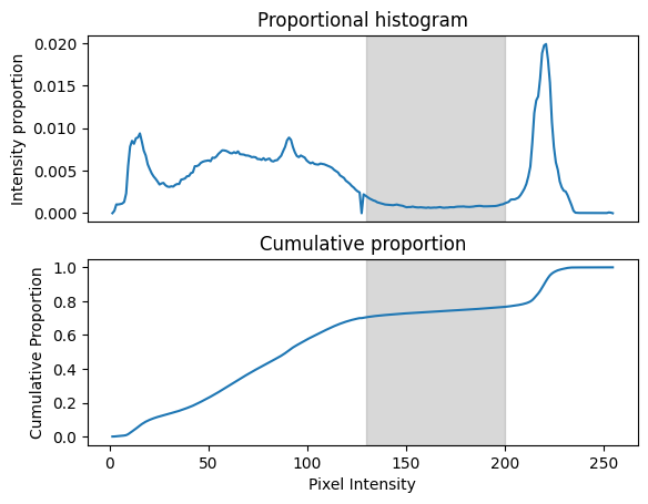
Now consider the low plateau in the proportional histogram between about pixel intensities of 130 to 200 (gray box). This corresponds to a plateau in the cumulative proportion in the same region, because there are relatively few pixels in the image within this wide range. In the original image there is a fairly wide difference (of 70) between pixels at either end of this plateau. However, there is a small difference in cumulative density (less than 0.1) for pixels between 130 and 200. If we replace the pixel values with the cumulative proportion values, this has the effect of compressing the image range devoted to difference along this plateau. Conversely, for parts of the intensity range where the there is a rapid change in cumulative proportion, replacing image intensity with cumulative proportion will have the effect of expanding the available image range for those image intensities. Thus the normalization has the effect of devoting greater image range to regions of rapid change in the original histogram.

Note

Why does histogram equalization work?

This note is for those of you who would like a more complete explanation for why the process of replacing the image count with the corresponding value from the cumulative distribution function (CDF) has the effect of making the image histogram flat.

Consider, say, a pixel with pixel intensity of 100. See the figures above for where this is in the image histogram.

We now look up this value (100) in the cumulative distribution function. As you can see in the figures above, the value is about 0.6. By definition, the 0.6 value means that 60% of the image intensity values are less than or equal to this value (of 100). Therefore, when we have replaced the pixel value of 100 with the CDF value of 0.6, we have made it such that there are exactly 60% of the (new, CDF-derived) pixel values less than or equal to the new value.

Have a look at this explanation, and in particular, the last graph on that page. You may be able to see that, by doing the operation above, we have made the CDF of the new values be a diagonal straight line (as in the graph on that page), and therefore, we have made the proportional histogram (that we can also call the Probability Density Function) be flat, with the image intensity divided into even bins.

The Numpy implementation of histogram equalisation has changed the dtype of the image because we have replaced values ranging from 1 to 255 with proportions ranging from 0 to 1:

# The `dtype` and `min`/`max` values of the original image.
show_attributes(eagle)

Type: <class 'numpy.ndarray'>
dtype: uint8
Shape: (2019, 1826)
Max Pixel Value: 255
Min Pixel Value: 1

# The `dtype` and `min`/`max` values of the filtered image.
show_attributes(equalised_hist)

Type: <class 'numpy.ndarray'>
dtype: float64
Shape: (3686694,)
Max Pixel Value: 1.0
Min Pixel Value: 0.0

This is important to be aware of, but we can easily convert back to the original dtype using the relevant function from ski.util. Speaking of ski, lets look at how to apply this filter in skimage in the next section…

Histogram equalisation in skimage

As usual, skimage makes it easy to implement this filter, in just a single line of code. We just pass our eagle image to the ski.exposure.equalize_hist() function, and it will carry out all the operations we saw above:

# Equalise `eagle` using `skimage.
eagle_equalized_with_ski = ski.exposure.equalize_hist(eagle)

# Generate the plot.
plt.figure(figsize=(14, 8))
plt.subplot(2, 2, 1)
plt.imshow(eagle)
plt.title('Original Image')
plt.subplot(2, 2, 2)
plt.hist(eagle.ravel(), bins=128)
plt.title('Original Histogram')
plt.subplot(2, 2, 3)
plt.imshow(eagle_equalized_with_ski)
plt.title('Equalised Image (via `skimage`)')
plt.subplot(2, 2, 4)
plt.hist(eagle_equalized_with_ski.ravel())
plt.title('Equalised Histogram (via `skimage`)')
plt.tight_layout();

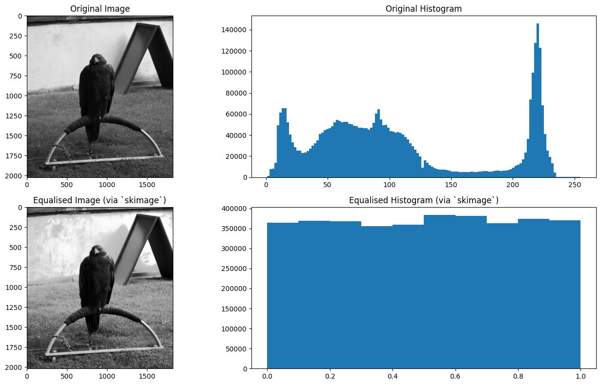
Easy-peasy. If you consult the documentation for ski.exposure.equalize_hist(), you notice that by default, it uses 256 bins. In fact, for the nbins optional argument, the documentation states that it will be ignored for integer data. This is so the “indexing trick” that we saw above can be performed.

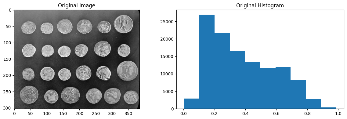
It is no problem to use this filter with float image data however - the principle is the same pixel intensities get mapped to their corresponding cumulative proportion. Only now this occurs without the neat indexing trick, there is just an intermediate (boring!) step in the mapping. We demonstrate this below with the coins image from ski.data:

# Import the `coins` image.
coins = ski.data.coins()

# Convert to `float64` `dtype`.
coins_as_float = ski.util.img_as_float64(coins)

# Show the image, the histogram of the image, and the attributes of the image.
plt.figure(figsize=(12, 4))
plt.subplot(1, 2, 1)
plt.imshow(coins_as_float)
plt.title('Original Image')
plt.subplot(1, 2, 2)
plt.hist(coins_as_float.ravel())
plt.title('Original Histogram')
plt.tight_layout();
show_attributes(coins_as_float)

Type: <class 'numpy.ndarray'>
dtype: float64
Shape: (303, 384)
Max Pixel Value: 0.99
Min Pixel Value: 0.0

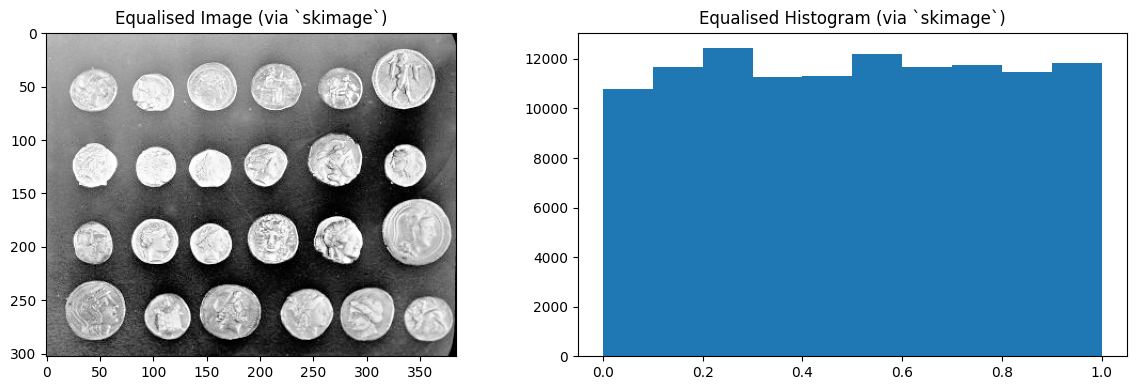
# Equalise the histogram.
coins_as_float_equalised_with_ski = ski.exposure.equalize_hist(coins_as_float)

# Show the image, the histogram of the image, and the attributes of the image.
plt.figure(figsize=(12, 4))
plt.subplot(1, 2, 1)
plt.imshow(coins_as_float_equalised_with_ski)
plt.title('Equalised Image (via `skimage`)')
plt.subplot(1, 2, 2)
plt.hist(coins_as_float_equalised_with_ski.ravel())
plt.title('Equalised Histogram (via `skimage`)')
plt.tight_layout();
show_attributes(coins_as_float_equalised_with_ski)

Type: <class 'numpy.ndarray'>
dtype: float64
Shape: (303, 384)
Max Pixel Value: 1.0
Min Pixel Value: 0.0

Summary

This page has shown a local filter (the median filter) and a non-local filter (histogram equalisation) which do not use kernel filtering to perform their filtering operations. On the next page we will introduce another method for modifying pixels based on a footprint.

References

Adapted from:

• Jan Erik Solem on histogram equalisation

• Jungletronics on histogram equalisation in OpenCV