Morphology#
Note
This tutorial is adapted from “Image manipulation and processing using NumPy and SciPy” by Emmanuelle Gouillart and Gaël Varoquaux, and “scikit-image: image processing” by Emmanuelle Gouillart. Please see the References section at the end of the page for other sources and resources.
Morphology is the
mathematical study of shapes and has numerous applications in image processing.
As such, Scikit-image has a dedicated module (ski.morphology) for associated
functions.
We have already encountered footprints and kernels on earlier pages. A footprint is a binary array defining a certain shape - you can think of it as a “template” — which is used to define the “neighborhood” of pixels which an image processing operation affects. As you remember, a kernel is a footprint containing weights. We might consider kernels as specialized footprints.
Note
Footprints and structuring elements
You will see other tutorials refer to footprints as structuring elements or structural elements. We stick to “footprint” here for compatibility with the Scikit-image terminology, but a footprint is identical in meaning to structuring/structural element.
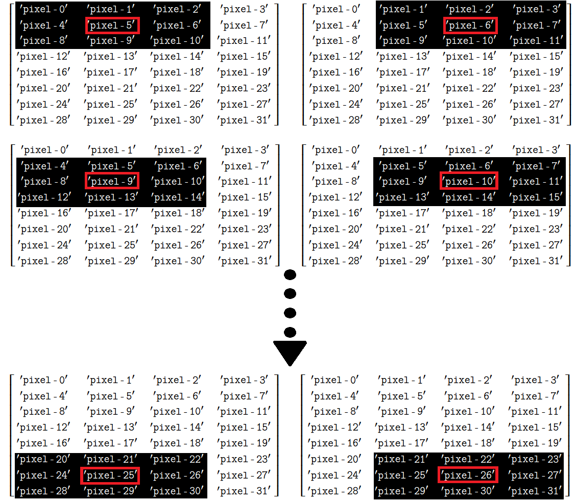
When applying our familiar mean filter, a (say) (3, 3) footprint can be applied as a square which affects 9 pixels - we might alter the image by centering this footprint over every pixel, and replacing each pixel with the mean of the other pixels in its “neighborhood”, for instance:
You will also recall that we need a strategy for pixels at the edge of the image, where we center the footprint on a pixel where part of the footprint “falls off” the edge of the image:
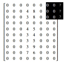
Options here including “padding” the empty footprint locations with a repeated value (like 0), or just duplicating the existing pixels at the edge of the image.
We have seen footprints and kernels applied during filtering operations,
courtesy of the ski.filters module. Morphological operations also make use of
footprints. As you remember, footprints (but not kernels) are binary (contain
only True / False or 0 / 1).
Morphology and footprints#
The fundamental operations of morphological image processing are erosion and dilation.
As you are about to see, basic morphological operations work on shapes within images by:
Choosing a footprint of a specific shape. This footprint acts as a “probe”, which scans over the image, centering on each pixel. The relationship between the probe and a given region of the image determines whether (and what) changes will be applied to that region.
Common footprint / function filtering operations applied via this probe are:
the
minimumfunction, to do an operation called erosion orthe
maximumfunction, to do an operation called dilation orsome combination of these.
The primary new thing we see in morphology, compared to our previous filters,
is the increased importance of the shape defined by the binary footprint.
Just to note, here we mean shape in the sense of square, diamond, triangle
etc., not shape in the sense of the Numpy
shape
attribute. Morphological operations alter regions of the image based on the
shape of the footprint, and so the specific shape of the footprint has a large
impact on the result of morphological operations. In addition, the
morphological operations covered on this page introduce the use of minimum
and maximum functions in footprint / function filters.
Therefore, morphology uses filters and crafted footprints to allow us to tune our filtering to the shape (…or, well, morphology) of features within the image.
Erosion is footprint / function filtering with minimum#
Let us leap ahead to show you the morphological operation of erosion.
As we said above, erosion is the application of a footprint / function filter,
where the function is minimum.
import skimage as ski
import numpy as np
import matplotlib.pyplot as plt

# A custom function for displaying image attributes.
from skitut import show_attributes

# A custom function to show original and altered images side-by-side.
from skitut import show_both

# Set 'gray' as the default colormap
plt.rcParams['image.cmap'] = 'gray'
The morphology (shape) part of erosion, is the choice of a footprint to identify the shape you are interested in, within the image.
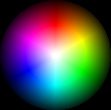
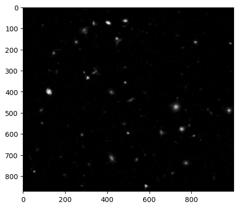
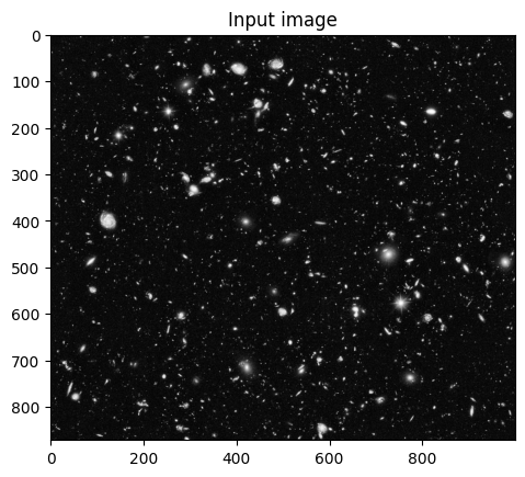
For example, consider this image — the blue channel of an image from the Hubble Space Telescope:
# Blue channel of Hubble image, as uint8
hubble_blue = ski.data.hubble_deep_field()[:, :, 2]
# As uint8 integer image type.
hubble_blue_ubyte = ski.util.img_as_ubyte(hubble_blue)
plt.imshow(hubble_blue_ubyte);

There are a small number of bright, large stars in this field, and a much larger number of smaller stars.
We might want to keep the larger disk-shaped objects in this image (brighter stars), and suppress the smaller objects.
We can do this by first specifying a disk as our footprint — identifying the shape of the local neighborhood:
# Our footprint is a disk of radius 5 pixels.
disk_5 = ski.morphology.disk(radius=5)
disk_5
array([[0, 0, 0, 0, 0, 1, 0, 0, 0, 0, 0],
       [0, 0, 1, 1, 1, 1, 1, 1, 1, 0, 0],
       [0, 1, 1, 1, 1, 1, 1, 1, 1, 1, 0],
       [0, 1, 1, 1, 1, 1, 1, 1, 1, 1, 0],
       [0, 1, 1, 1, 1, 1, 1, 1, 1, 1, 0],
       [1, 1, 1, 1, 1, 1, 1, 1, 1, 1, 1],
       [0, 1, 1, 1, 1, 1, 1, 1, 1, 1, 0],
       [0, 1, 1, 1, 1, 1, 1, 1, 1, 1, 0],
       [0, 1, 1, 1, 1, 1, 1, 1, 1, 1, 0],
       [0, 0, 1, 1, 1, 1, 1, 1, 1, 0, 0],
       [0, 0, 0, 0, 0, 1, 0, 0, 0, 0, 0]], dtype=uint8)
# Footprint as image.
plt.imshow(disk_5);
This will be our footprint when applying a minimum function, from ski.filter.rank, like this:
hubble_eroded = ski.filters.rank.minimum(hubble_blue_ubyte, disk_5)
plt.imshow(hubble_eroded);
This is the algorithm for erosion, one of the two basic operations in morphology (the other being dilation).
You will see above, the minimum filtering with the disk footprint has the effect of keeping areas which are disks of the given size or bigger, and suppressing areas which have objects of smaller size. The next section explains how this works, using binary images as examples.
We have said that erosion is the process of applying a footprint / function filter, where the function is minimum (as above). Just to show this is the case, here we use the ski.morphology.erosion function to apply the same operation, and get exactly the same result:
hubble_eroded_again = ski.morphology.erosion(hubble_blue_ubyte, disk_5)
# We get exactly the result we got by applying the minimum filter above.
np.all(hubble_eroded_again == hubble_eroded)
np.True_
With that example, let us return to a discussion of the erosion (footprint / minimum) algorithm.
Footprints as template shapes#
Because morphological operations are part of image processing, they involve the modification of array pixel values. In morphological operations, the footprint guides changes to pixel values depending upon the relationship between the shape of the footprint and the shape of the pixels in the “neighborhood” of the footprint.
The footprint is centered once on every pixel in an image, and this central pixel is modified (or not) depending upon the relationship between the shape of the footprint and the shape described by the pixel values in that neighborhood. Changing the shape of the footprint will change these relationships, and hence will alter the output of the operation.
Note
Footprints and centering
We asserted above that we center the footprint on each pixel in the image, and
this by far the most common procedure. However, you can ask Scikit-image or
Scipy ndimage to offset the footprint centering by a given number of pixels. See the corresponding help for the Scikit-image and ndimage functions for detail on how to do this.
Erosion on a binary image#
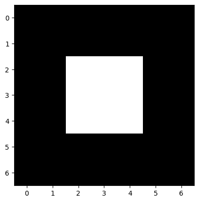
It can be easier to think of erosion (and dilation) in terms of their effects on simple binary (True / False, 1 / 0) images.
# Make a binary square.
square = np.array([[0, 0, 0, 0, 0, 0, 0],
                   [0, 0, 0, 0, 0, 0, 0],
                   [0, 0, 1, 1, 1, 0, 0],
                   [0, 0, 1, 1, 1, 0, 0],
                   [0, 0, 1, 1, 1, 0, 0],
                   [0, 0, 0, 0, 0, 0, 0],
                   [0, 0, 0, 0, 0, 0, 0]], dtype=np.uint8)
plt.imshow(square);
Let’s get fancy and ostentatious now, and invest in some diamonds, by which we
mean, let’s use ski.morphology.diamond() to construct a new footprint:
# Create a `diamond` footprint.
# Changing `radius` will change the size of the diamond.
diamond = ski.morphology.diamond(radius=1)
diamond
array([[0, 1, 0],
       [1, 1, 1],
       [0, 1, 0]], dtype=uint8)
plt.matshow(diamond);
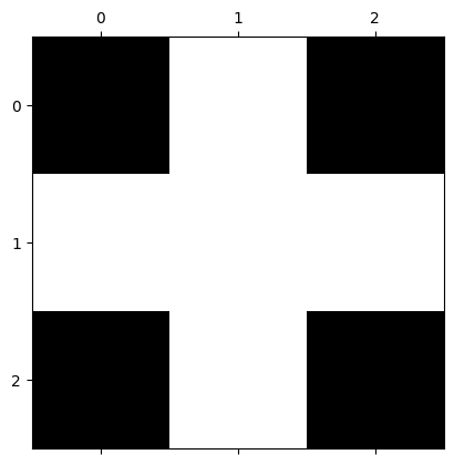
Using ski.morphology.diamond(radius=1) gives us a diamond shaped footprint of
shape (3, 3). We’d call it a “cross” but “diamond” is the canonical term…
Be assured that it will look more diamond-like (diamond-y?) when set to
a bigger radius…:
diamond.shape
(3, 3)
As you read above, erosion proceeds by applying the following algorithm at each pixel of the image.
Placing the footprint over the pixel and
Selecting the pixel values under the footprint (where the footprint is 1 / True) and
Setting the output value at the given pixel to the minimum of the selected values.
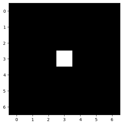
Here we erode our binary square using ski.morphology.erosion(). We could
equivalently have used ski.filter.rank.minimum. In either case, we use the
footprint argument to specify our footprint:
# Erode our image.
eroded_square = ski.morphology.erosion(square,
                                       footprint=diamond)
# Show the result.
eroded_square
array([[0, 0, 0, 0, 0, 0, 0],
       [0, 0, 0, 0, 0, 0, 0],
       [0, 0, 0, 0, 0, 0, 0],
       [0, 0, 0, 1, 0, 0, 0],
       [0, 0, 0, 0, 0, 0, 0],
       [0, 0, 0, 0, 0, 0, 0],
       [0, 0, 0, 0, 0, 0, 0]], dtype=uint8)
What has happened here? For the purposes of the erosion operation, we can think of our diamond footprint as being a bit
like a weird crosshair/reticle of
a gun. We “target” this crosshair on a given
array pixel.
When we apply the footprint to each pixel in the image, call the pixels under the footprint — the pixel neighborhood. Because we are eroding, the central pixel will be lowered to the value of the lowest pixel in its neighborhood.
In our specific case the pixel neighbourhood is the set of pixels in the image which fall under the “crosshair” shape of the footprint. In other words, the neighbourhood is the set of image pixels under the elements of the footprint which equal 1:
# Here is our footprint...
diamond
array([[0, 1, 0],
       [1, 1, 1],
       [0, 1, 0]], dtype=uint8)
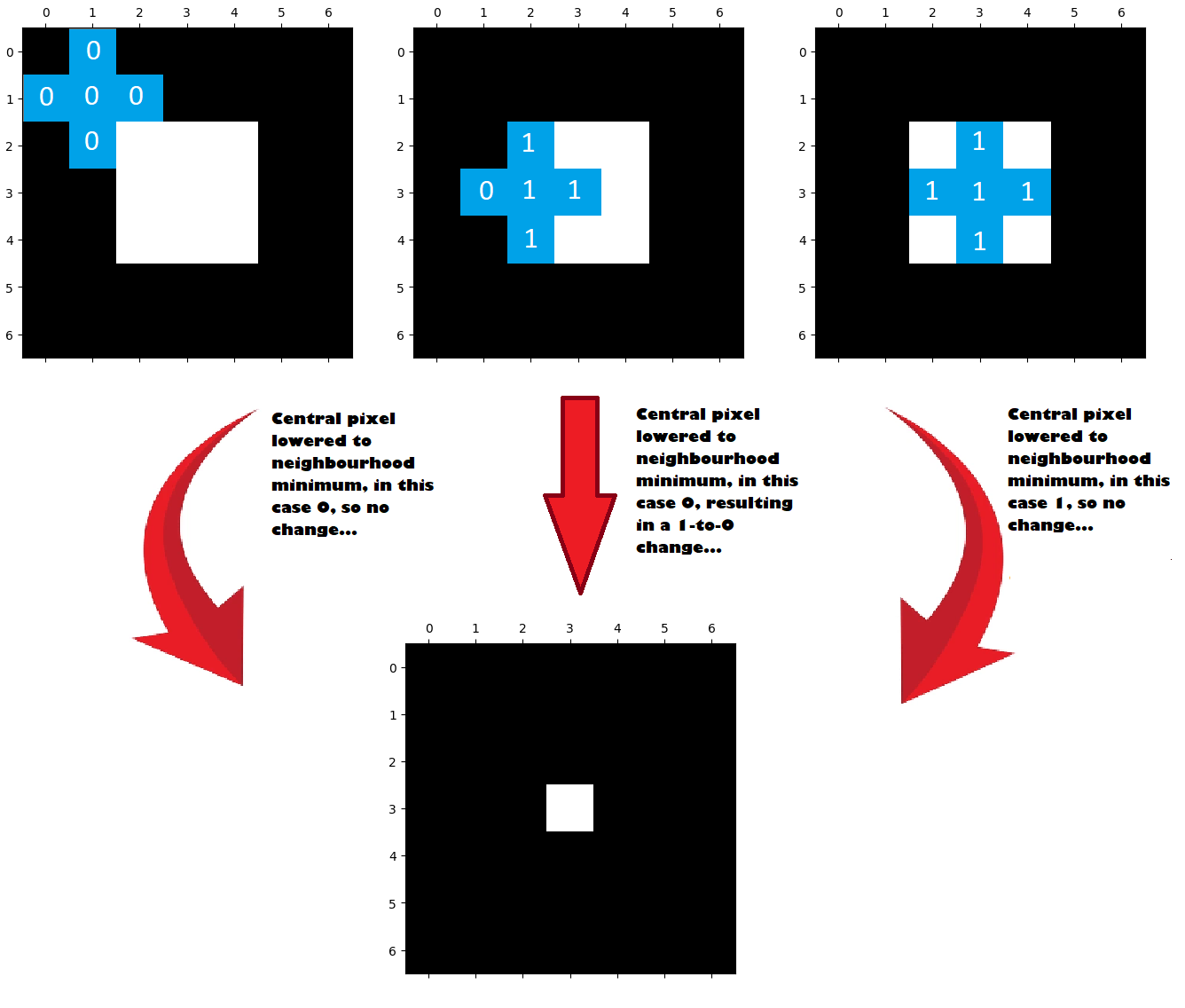
Because we are eroding, and because our square array contains only 1s and 0s,
the output pixels will be 1 only if all pixels in the local
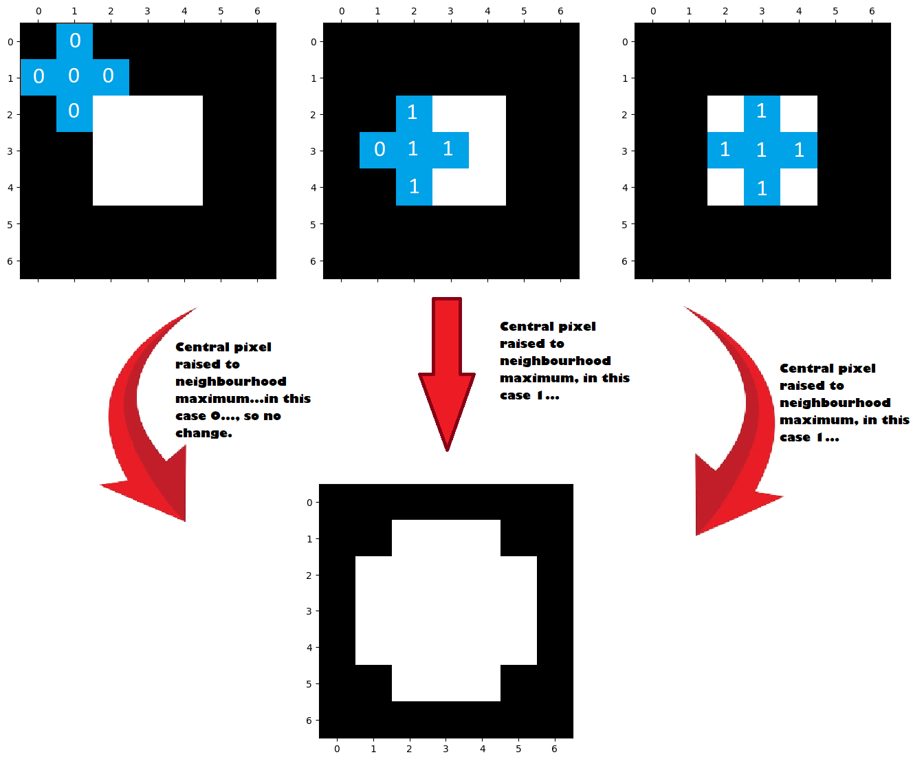
neighborhood are 1, and 0 otherwise. The image below shows the diamond
footprint being applied to three different central pixels. We we use blue squares to represent the footprint, with white text showing what value is in the image array at that location.
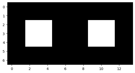
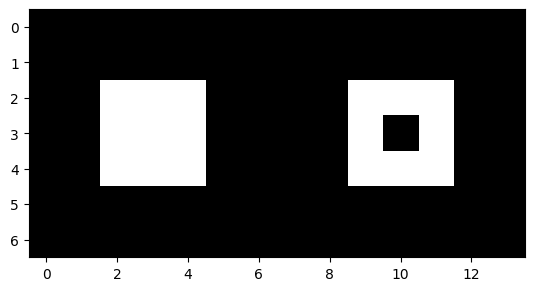
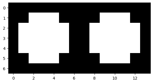
Let’s repeat this erosion process with two square arrays concatenated
together.
What do you think will happen when we erode them using the diamond
footprint? Try to predict before you check:
# `concatenate` two `square` arrays.
two_squares = np.concatenate([square, square], axis=1)
plt.imshow(two_squares);
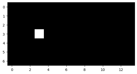
# Perform the erosion.
eroded_two_squares = ski.morphology.erosion(two_squares, diamond)
eroded_two_squares
array([[0, 0, 0, 0, 0, 0, 0, 0, 0, 0, 0, 0, 0, 0],
       [0, 0, 0, 0, 0, 0, 0, 0, 0, 0, 0, 0, 0, 0],
       [0, 0, 0, 0, 0, 0, 0, 0, 0, 0, 0, 0, 0, 0],
       [0, 0, 0, 1, 0, 0, 0, 0, 0, 0, 1, 0, 0, 0],
       [0, 0, 0, 0, 0, 0, 0, 0, 0, 0, 0, 0, 0, 0],
       [0, 0, 0, 0, 0, 0, 0, 0, 0, 0, 0, 0, 0, 0],
       [0, 0, 0, 0, 0, 0, 0, 0, 0, 0, 0, 0, 0, 0]], dtype=uint8)
# Plot the result of the erosion.
plt.imshow(eroded_two_squares);
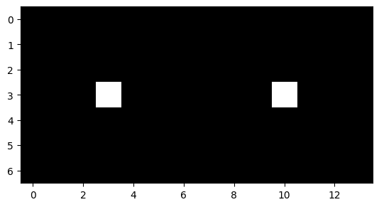
What happened here? Well, only two pixels have 1 as their neighbourhood minimum - the pixels at the center of each white square. This illustration below shows what happened:
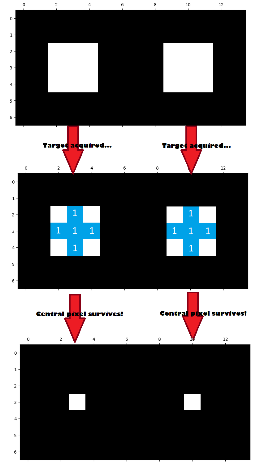
All other “neighborhoods” had at least one 0 in them, and so their central pixels were lowered to 0, resulting in 1-to-0 changes if the central pixel had a value of 1.
One way to think of this is that the erosion footprint is “searching” for areas of the image which “match” its shape. For a central pixel with a value of 1 to “survive”, all the values in its neighbourhood must also be 1. In this instance, the neighbourhood “matches” the footprint because the neighbourhood has 1’s everywhere the footprint has 1’s. If at least one value in the neighbourhood does not match the shape of the 1’s in the footprint (e.g. there is a 0 anywhere under the “crosshair”), then the output pixel value gets set to 0.
Let’s alter our image array slightly, to see how this affects the erosion operation with our diamond footprint. We will place a black array pixel inside the right-hand white square:
# A modified array.
square_the_circle = np.array([[0, 0, 0, 0, 0, 0, 0, 0, 0, 0, 0, 0, 0, 0],
                               [0, 0, 0, 0, 0, 0, 0, 0, 0, 0, 0, 0, 0, 0],
                               [0, 0, 1, 1, 1, 0, 0, 0, 0, 1, 1, 1, 0, 0],
                               [0, 0, 1, 1, 1, 0, 0, 0, 0, 1, 0, 1, 0, 0],
                               [0, 0, 1, 1, 1, 0, 0, 0, 0, 1, 1, 1, 0, 0],
                               [0, 0, 0, 0, 0, 0, 0, 0, 0, 0, 0, 0, 0, 0],
                               [0, 0, 0, 0, 0, 0, 0, 0, 0, 0, 0, 0, 0, 0]],
                               dtype="uint8")

plt.imshow(square_the_circle);
Before looking at the output of the cell below, try to think carefully about
how you think this will affect the erosion operation, using the (3, 3)
diamond footprint. Picture what will happen on the black pixel in the center
of the right-hand square.
Scroll down to the output of the cell below to see if your prediction was correct:
eroded_square_the_circle = ski.morphology.erosion(square_the_circle, diamond)
plt.imshow(eroded_square_the_circle);
Ok, so now the whole right-hand square got taken out. Brutal.
Why did this happen? The cell below illustrates, using green ticks for “matches” between the footprint and the pixel “neighborhood”, and red X’s for “clashes” between the footprint and the pixel “neighborhood”.
Remember that any “clash” means the central pixel “dies” (gets set to 0); a “match” means the central pixel “survives” (gets set to 1).
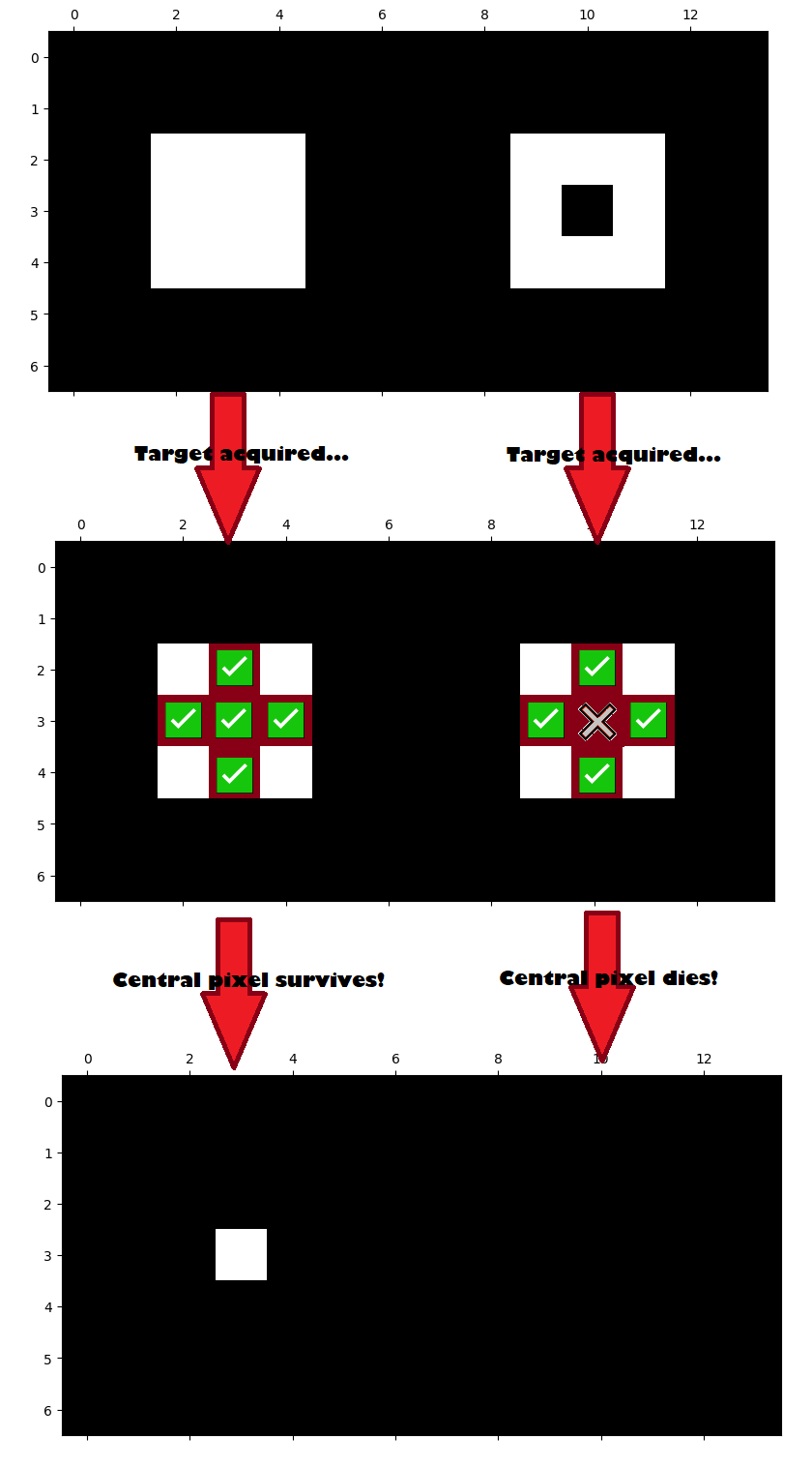
Think of erosion as searching for, and maintaining, areas matching the footprint shape, while suppressing areas not of that shape.
Dilation#
The other foundational operation in morphological image processing is dilation.
Dilation is nothing but a footprint / function filter, where the function is
maximum rather than minimum.
Dilation works in the same way as erosion, or any other footprint / function filter, in terms of centering a footprint on each pixel, to select the pixel local neighborhood. It takes the maximum of the local pixel values. Wherever the footprint “lands” the central pixel will be raised to the neighbourhood maximum.
Let’s dilate the square array to illustrate:
# Show the `square` array.
square
array([[0, 0, 0, 0, 0, 0, 0],
       [0, 0, 0, 0, 0, 0, 0],
       [0, 0, 1, 1, 1, 0, 0],
       [0, 0, 1, 1, 1, 0, 0],
       [0, 0, 1, 1, 1, 0, 0],
       [0, 0, 0, 0, 0, 0, 0],
       [0, 0, 0, 0, 0, 0, 0]], dtype=uint8)
plt.imshow(square);
Next we use ski.morphology.dilation() to dilate the image. We could,
equivalently, use the ski.filter.rank.maximum function. Again, we will use
diamond as our footprint:
# Perform the dilation.
dilated_square = ski.morphology.dilation(square,
                                         footprint=diamond)
dilated_square
array([[0, 0, 0, 0, 0, 0, 0],
       [0, 0, 1, 1, 1, 0, 0],
       [0, 1, 1, 1, 1, 1, 0],
       [0, 1, 1, 1, 1, 1, 0],
       [0, 1, 1, 1, 1, 1, 0],
       [0, 0, 1, 1, 1, 0, 0],
       [0, 0, 0, 0, 0, 0, 0]], dtype=uint8)
plt.imshow(dilated_square);
Again, here we use blue squares to represent the footprint, with white text showing the value in the array at that location. Remember, dilation will raise the central pixel to the neighbourhood maximum.
So, if the values under the footprint are all 0, then the central pixel will remain as 0.
If there are any 1 values under the footprint, then the central value will be raised to 1:
What do you think will happen if we dilate the square_the_circle array image
shown below, using the diamond footprint?
Try to predict before checking:
# Show the array.
square_the_circle
array([[0, 0, 0, 0, 0, 0, 0, 0, 0, 0, 0, 0, 0, 0],
       [0, 0, 0, 0, 0, 0, 0, 0, 0, 0, 0, 0, 0, 0],
       [0, 0, 1, 1, 1, 0, 0, 0, 0, 1, 1, 1, 0, 0],
       [0, 0, 1, 1, 1, 0, 0, 0, 0, 1, 0, 1, 0, 0],
       [0, 0, 1, 1, 1, 0, 0, 0, 0, 1, 1, 1, 0, 0],
       [0, 0, 0, 0, 0, 0, 0, 0, 0, 0, 0, 0, 0, 0],
       [0, 0, 0, 0, 0, 0, 0, 0, 0, 0, 0, 0, 0, 0]], dtype=uint8)
plt.imshow(square_the_circle);
Let’s see how good your prediction was:
# Dilate the `square_the_circle` array, and show the result.
dilated_square_the_circle = ski.morphology.dilation(square_the_circle,
                                                    footprint=diamond)
plt.imshow(dilated_square_the_circle);
Why did this happen? The image below explains:
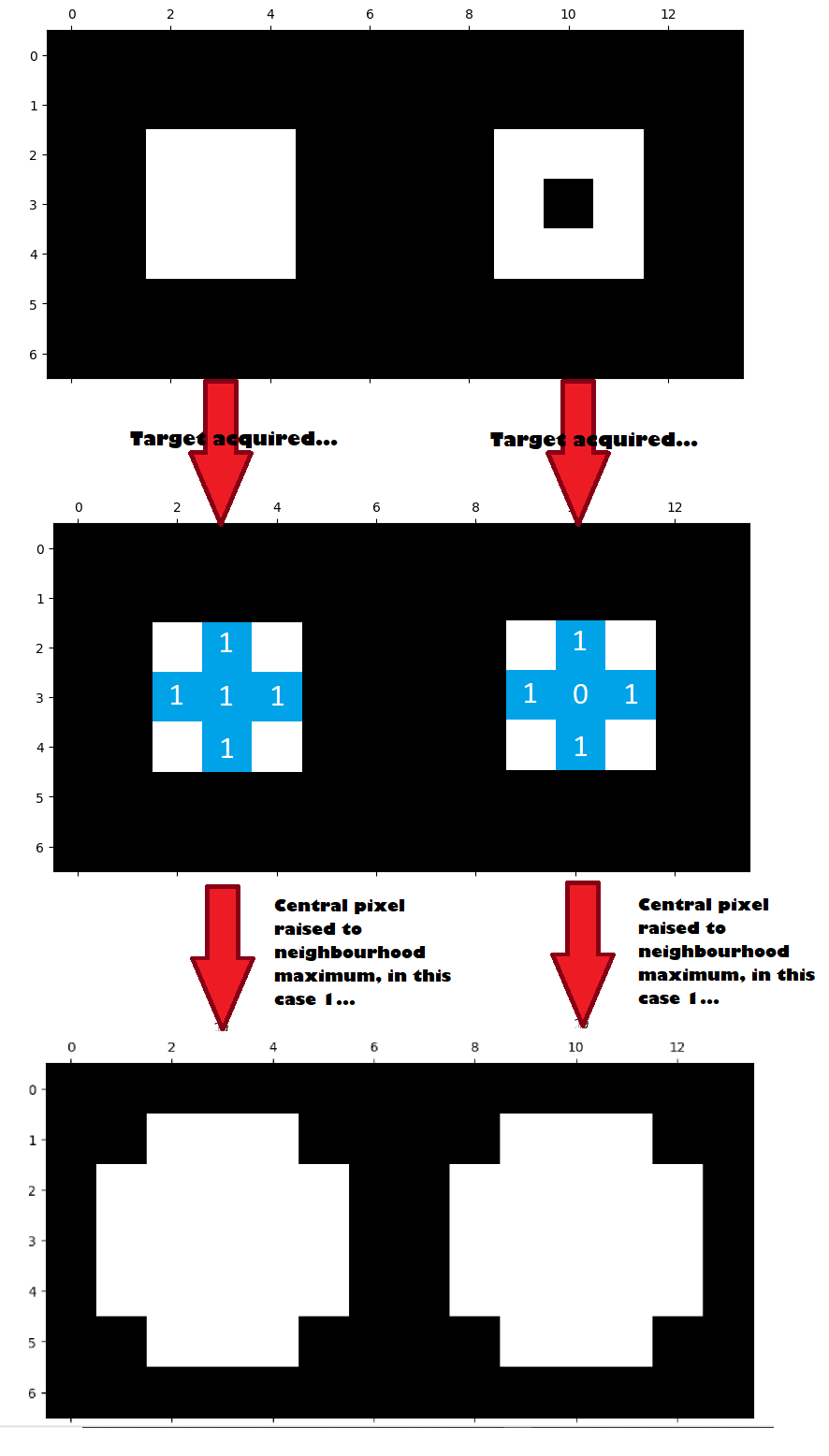
For erosion, all of the central pixels in the right-hand square get lowered to their neighborhood minimum, in this case 0, and so they “die” and fade into the black background.
For dilation, central pixels get raised to the neighborhood maximum, which in this case is 1. So the black central pixel is brightened to white.
Think of dilation as extending bright areas with the footprint shape.
Another way of thinking of this is:
Erosion enlarges dark regions and shrinks bright regions.
Dilation enlarges bright regions and shrinks dark regions.
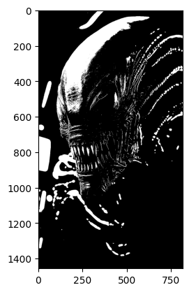
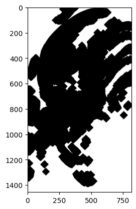
Morphology using more complex images#
Let’s apply some of this to more complex images. Fittingly, we will use a terrifying picture of a Xenomorph, which at the time of writing Wikipedia defines as “a fictional endoparasitoid extraterrestrial species that serves as the main antagonist of the Alien and Alien vs. Predator franchises”. Yikes.
# Photo by Stockcake
# - https://stockcake.com/i/alien-head-close-up_1354662_1093149
xenomorph = ski.io.imread("images/xenomorph.jpg", as_gray=True)
# Convert to binary.
xenomorph = ski.util.img_as_bool(xenomorph).astype(int)

# Show the "raw" array.
xenomorph
array([[0, 0, 0, ..., 0, 0, 0],
       [0, 0, 0, ..., 0, 0, 0],
       [0, 0, 0, ..., 0, 0, 0],
       ...,
       [0, 0, 0, ..., 0, 0, 0],
       [0, 0, 0, ..., 0, 0, 0],
       [0, 0, 0, ..., 0, 0, 0]], shape=(1456, 816))
plt.imshow(xenomorph);
# Show the attributes of `xenomorph`.
show_attributes(xenomorph)
Type: <class 'numpy.ndarray'>
dtype: int64
Shape: (1456, 816)
Max Pixel Value: 1
Min Pixel Value: 0
Scary, especially as a binary image, but not quite as scary as the smiley image we made that still haunts our dreams.
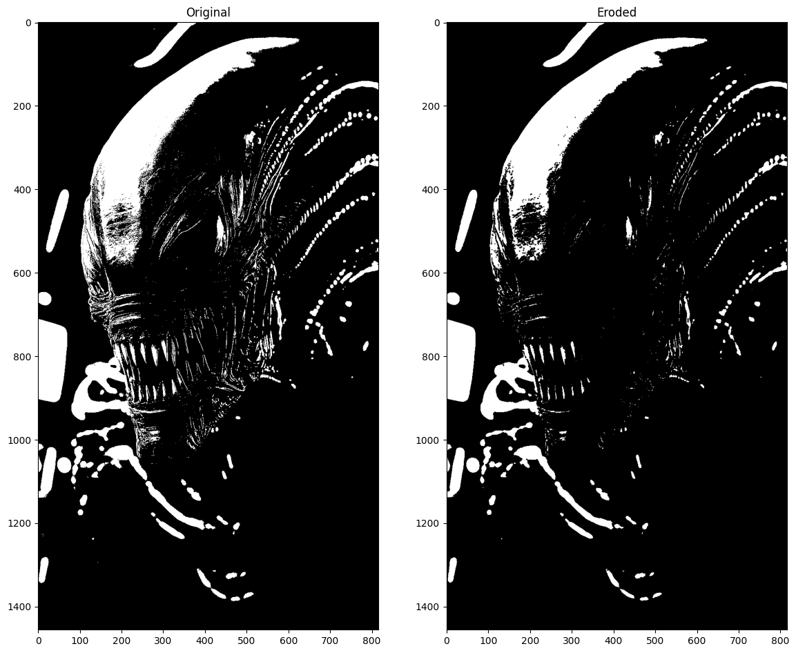
True to form, eroding this image using the diamond footprint increases the
size of dark regions:
# Erode the xenomorph.
xeno_binary_ero_rad_1_diamond = ski.morphology.erosion(xenomorph,
                                                       footprint=diamond)

# Show the result.
show_both(xenomorph, xeno_binary_ero_rad_1_diamond, "Eroded");
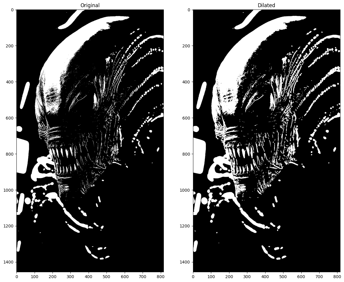
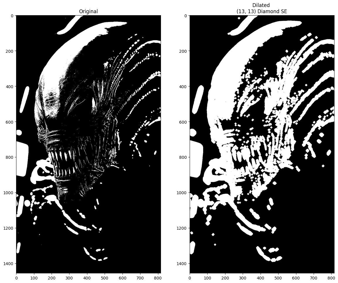
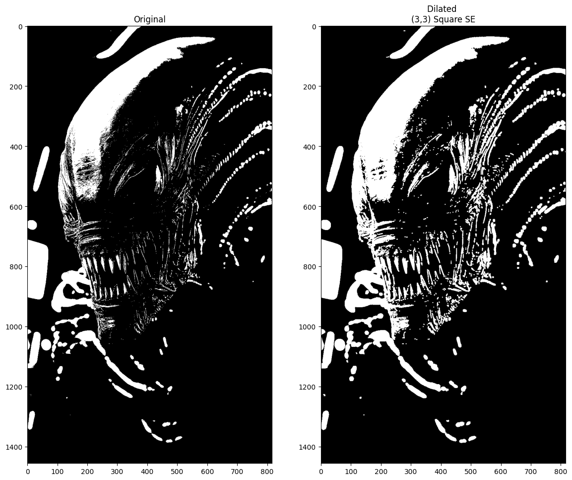
Whilst dilation increases the size of bright regions (creating a truly, truly terrifying image):
# Dilate the xenomorph.
xeno_binary_dilate_rad_1_diamond = ski.morphology.dilation(xenomorph,
                                                           footprint=diamond)

# Show the result.
show_both(xenomorph, xeno_binary_dilate_rad_1_diamond, "Dilated");
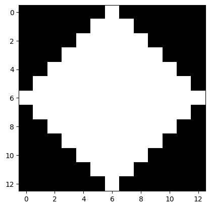
We can alter the size of the footprint to change the nature of the effect. The
exact change will be heavily dependent on the image array we are processing.
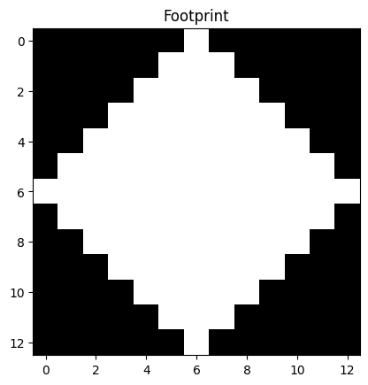
Here we create a diamond with radius=6:
# Create and show a larger diamond footprint.
diamond_6 = ski.morphology.diamond(radius=6)
diamond_6
array([[0, 0, 0, 0, 0, 0, 1, 0, 0, 0, 0, 0, 0],
       [0, 0, 0, 0, 0, 1, 1, 1, 0, 0, 0, 0, 0],
       [0, 0, 0, 0, 1, 1, 1, 1, 1, 0, 0, 0, 0],
       [0, 0, 0, 1, 1, 1, 1, 1, 1, 1, 0, 0, 0],
       [0, 0, 1, 1, 1, 1, 1, 1, 1, 1, 1, 0, 0],
       [0, 1, 1, 1, 1, 1, 1, 1, 1, 1, 1, 1, 0],
       [1, 1, 1, 1, 1, 1, 1, 1, 1, 1, 1, 1, 1],
       [0, 1, 1, 1, 1, 1, 1, 1, 1, 1, 1, 1, 0],
       [0, 0, 1, 1, 1, 1, 1, 1, 1, 1, 1, 0, 0],
       [0, 0, 0, 1, 1, 1, 1, 1, 1, 1, 0, 0, 0],
       [0, 0, 0, 0, 1, 1, 1, 1, 1, 0, 0, 0, 0],
       [0, 0, 0, 0, 0, 1, 1, 1, 0, 0, 0, 0, 0],
       [0, 0, 0, 0, 0, 0, 1, 0, 0, 0, 0, 0, 0]], dtype=uint8)
plt.imshow(diamond_6);
Applied to the xenomorph image in an erosion operation, this has some radical
results:
xeno_binary_ero_rad_6_diamond = ski.morphology.erosion(xenomorph,
                                                       footprint=diamond_6)
show_both(xenomorph,
          xeno_binary_ero_rad_6_diamond,
          "Eroded \n(13, 13) Diamond SE");
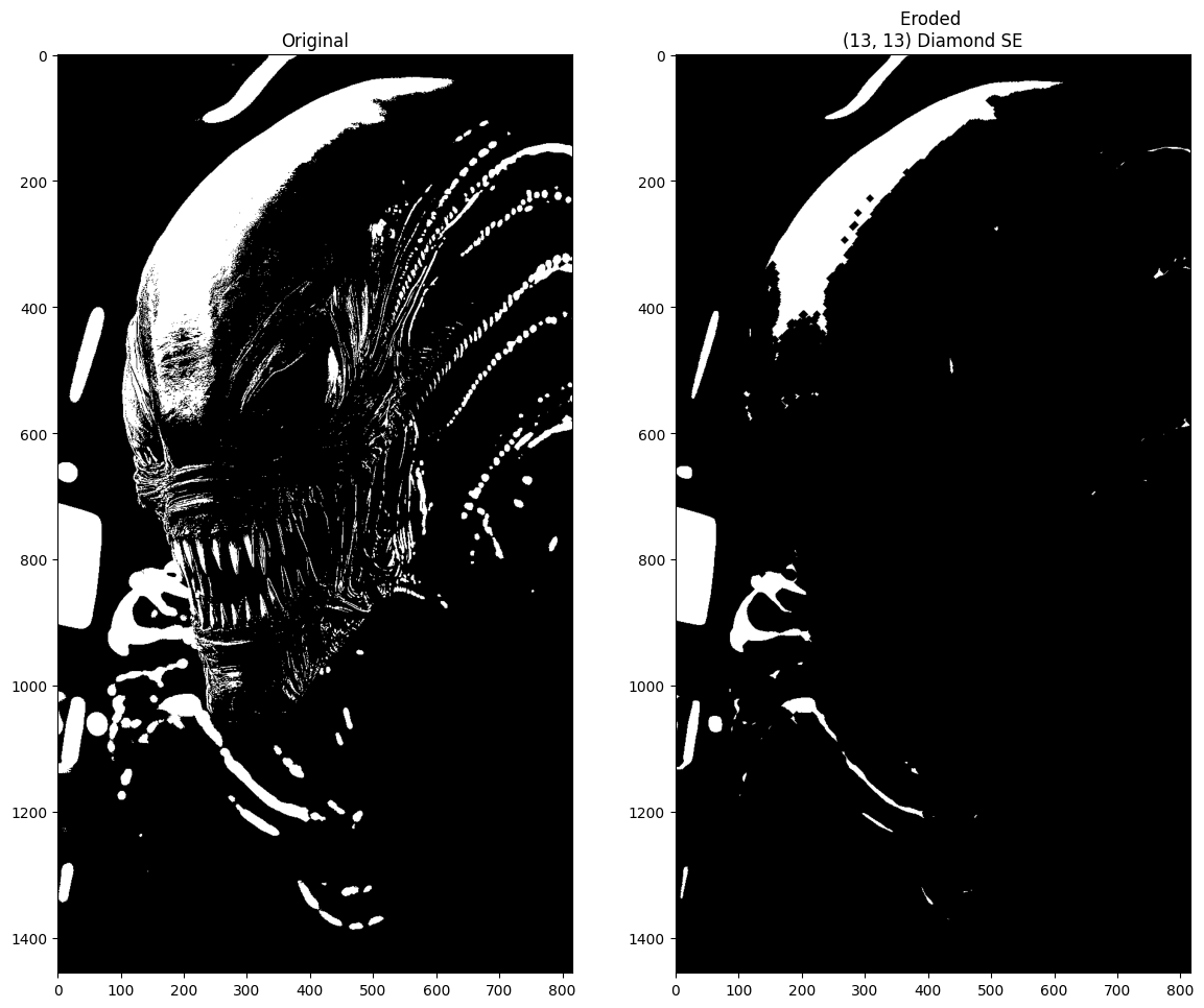
There are fewer areas for this large footprint where the all the values (and
therefore the minimum value) is high. Therefore, erosion leaves less central
pixels with relatively high values, than for a smaller footprint of the same
shape. For all the pixels where the local neighborhood includes at least one
low-value pixel, the erosion output is low-value, so the darker regions have
expanded substantially more than when we used a smaller diamond, which gave
more “matches”.
Dilation, again has the opposite effect of increasing brighter regions around regions that are already bright:
# Dilate the xenomorph with the `radius = 6` diamond.
xeno_binary_dilate_rad_6_diamond = ski.morphology.dilation(xenomorph,
                                                           footprint=diamond_6)
show_both(xenomorph,
          xeno_binary_dilate_rad_6_diamond,
          "Dilated \n(13, 13) Diamond SE");
Remember that the increased importance of shape is what makes morphological operations different to other footprint / function filtering operations. As a result, changing the shape of the footprint can alter the effect of a morphological operation, sometimes substantially.
Below we change the shape of the footprint - here we create a rectangle (Ok, a square) of shape (3, 3):
# A square footprint.
square_SE = ski.morphology.footprint_rectangle((3, 3))
square_SE
array([[1, 1, 1],
       [1, 1, 1],
       [1, 1, 1]], dtype=uint8)
This new footprint is the same shape as the kernels we used on the
filtering page. Below we use it to erode the xenomorph image:
# Erode the xenomorph (with the square footprint).
xeno_binary_ero_square = ski.morphology.erosion(xenomorph,
                                                footprint=square_SE)
show_both(xenomorph,
          xeno_binary_ero_square,
          "Eroded \n(3,3) Square SE");
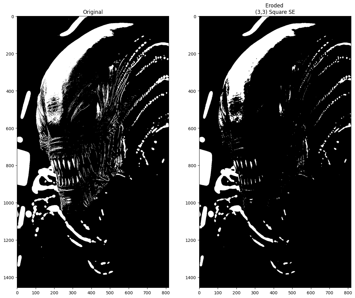
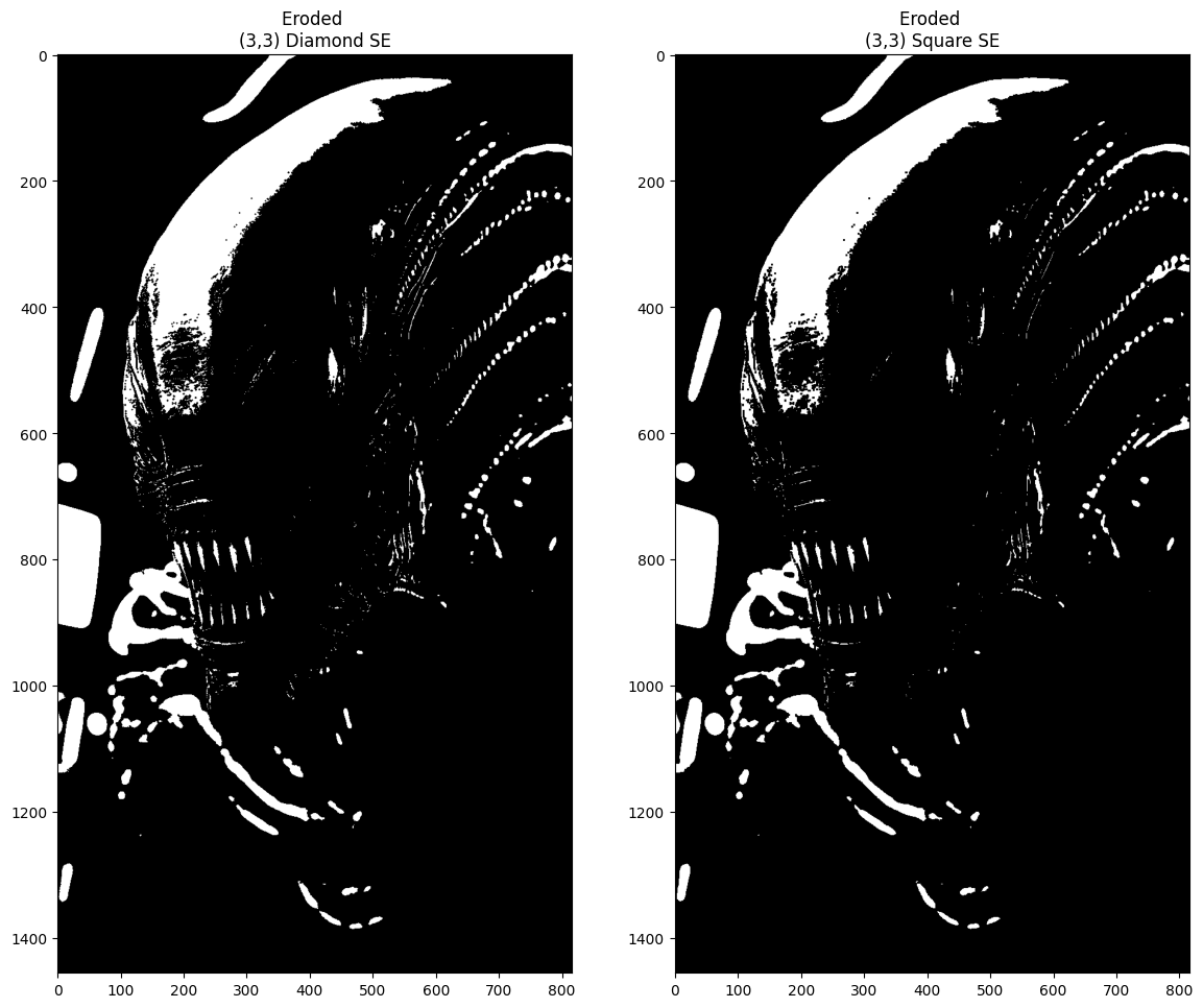
The difference here between eroding with a (3,3) diamond vs a (3,3) square is subtle, but changing the morphology (shape) of the probe changes the impact of the filtering operation. The output images are shown below - can you find regions where the different probes have resulted in different white pixels “surviving” each operation?:
show_both(xeno_binary_ero_rad_1_diamond,
          xeno_binary_ero_square,
          "Eroded \n(3,3) Square SE",
          "Eroded \n(3,3) Diamond SE");
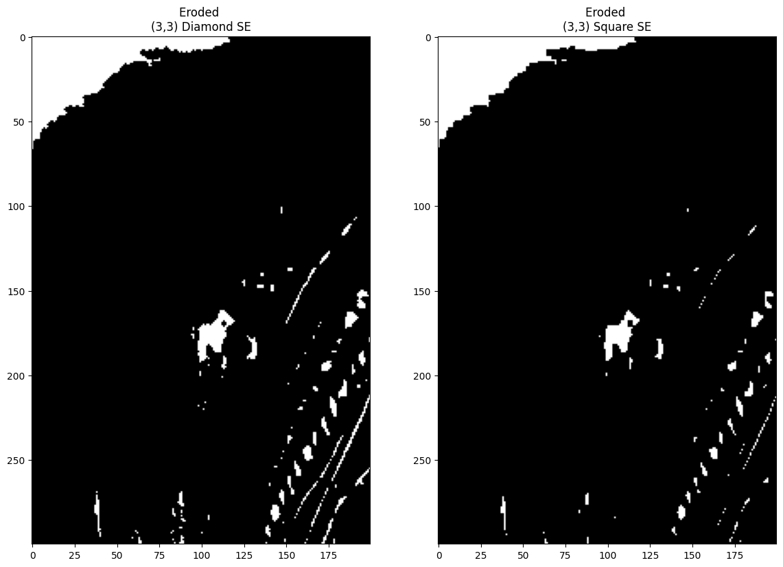
Below we use an indexing operation to “zoom in” on the same region in each image, for easier comparison. We can now see that changing the shape of the (3,3) probe (diamond vs square) alters which pixels “survive” the erosion:
show_both(xeno_binary_ero_rad_1_diamond[100:400,400:600],
          xeno_binary_ero_square[100:400,400:600],
          "Eroded \n(3,3) Square SE",
          "Eroded \n(3,3) Diamond SE");
By comparison, dilation with this new square footprint once more enlarges brighter regions, again with horrific results:
# Dilate the xenomorph, with the new footprint.
xeno_binary_dilate_square = ski.morphology.dilation(xenomorph,
                                                    footprint=square_SE)
show_both(xenomorph, xeno_binary_dilate_square, "Dilated \n(3,3) Square SE");
Changing the shape or size of the footprint will change the local pixel neighborhood, and therefore the degree and location of changes to the bright/dark regions, for both erosion and dilation. We are essentially looking for features of a certain shape (the shape of our footprint) in the image, and then dilating (increasing to neighborhood maximum) / eroding (decreasing to neighborhood minimum) on that basis.
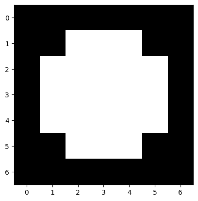
Exercise 27
Try to recreate the following image by processing xenomorph, using only
skimage morphological operations, as well as operations from the other
tutorials, from numpy, scipy and skimage:
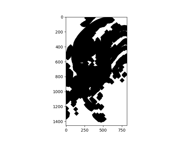
Look at the shape, the morphology of the features in the image - what shape and size footprint do you think you need? Do you think you need dilation or erosion?
For comparison, here is the original binarized image:
plt.imshow(xenomorph);
# YOUR CODE HERE
img = ...
Solution to Exercise 27
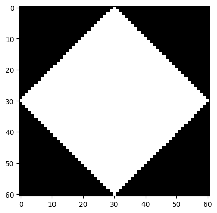
We promised earlier that the diamond footprint would get more diamond-like
when it is larger. To complete this exercise, you need big_diamond with
radius = 30:
# Expensive!
big_diamond = ski.morphology.diamond(radius=30)
plt.imshow(big_diamond);
Dilating with this big_diamond will give you the right outline, but the
wrong colors:
# Solution, part 1:
xeno_big_diamond = ski.morphology.dilation(xenomorph,
                                           footprint=big_diamond)
plt.imshow(xeno_big_diamond);
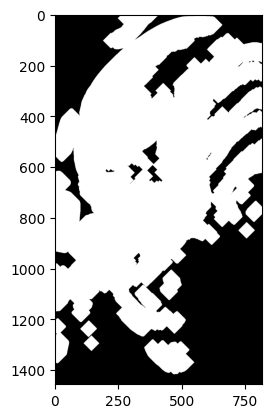
To get the target image, we need to invert the colors:
# Solution, part 2:
inverted_xeno_big_diamond = ski.util.invert(xeno_big_diamond)
plt.imshow(inverted_xeno_big_diamond);
Erosion and dilation on greyscale images#
For most of this tutorial we have used binary images to show erosion and dilation, but as you know the algorithm, it will be obvious how erosion and dilation apply to greyscale images.
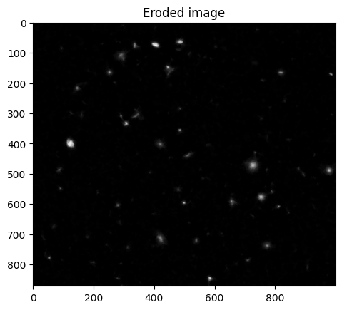
Erosion is the application of a footprint / minimum filter, so bright regions
matching the footprint shape will continue to be bright, but other regions,
including those at the edge of bright regions, will become dark (as they
acquire the minimum of the local neighborhood). You have already seen erosion
with a radius 6 disk applied to the Hubble Space Telescope image above. Let’s
apply the diamond_6 footprint to this image.
# The original image (blue channel of Hubble image).
plt.imshow(hubble_blue_ubyte);
plt.title('Input image');
# The footprint we will use.
plt.imshow(diamond_6)
plt.title('Footprint');
# Eroded image.
# We used the equivalent ski.filters.rank.minimum call previously.
hubble_eroded = ski.morphology.erosion(hubble_blue_ubyte, diamond_6)
plt.imshow(hubble_eroded)
plt.title('Eroded image');
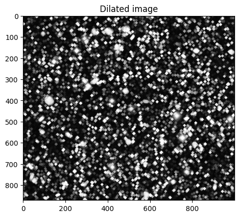
We can also apply dilation. Here pixels with any bright pixel in the local neighborhood become bright, so small bright objects will become larger.
# Dilated image.
hubble_dilated = ski.morphology.dilation(hubble_blue_ubyte, diamond_6)
plt.imshow(hubble_dilated)
plt.title('Dilated image');
Notice that you can think of erosion is dilation of the dark areas in the image, and dilation as erosion of the dark areas.
Opening and closing#
Opening and [closing](https://en.wikipedia.org/wiki/Closing_(morphology) are two other important morphological operations.
Opening is the result of:
Applying erosion to an image and then
Applying dilation to the result.
Closing is the result of
Applying dilation to an image and then
Applying erosion to the result.
Some reflection might reveal what kind of effects these will have.
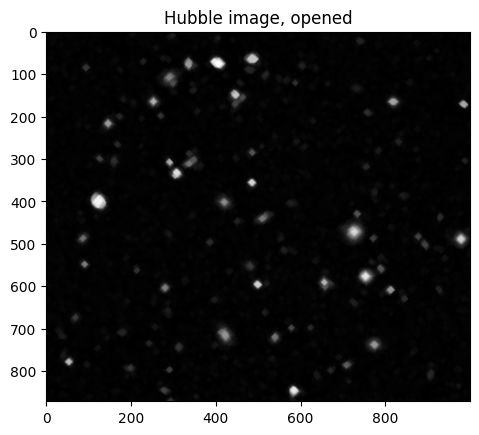
For opening, we are first trimming the image down to objects matching the footprint, and then expanding the remaining objects.
# Recalculate the eroded Hubble image.
hubble_eroded = ski.morphology.erosion(hubble_blue_ubyte, diamond_6)
# Calculate the opened image by dilating the eroded image.
hubble_opened = ski.morphology.dilation(hubble_eroded, diamond_6)
plt.imshow(hubble_opened)
plt.title('Hubble image, opened');
We asserted that opening was erosion followed by dilation, but you will want confirmation of this:
# Is ski.morphology.opening actually the same as dilation on erosion?
np.all(ski.morphology.opening(hubble_blue_ubyte, diamond_6) == hubble_opened)
np.True_
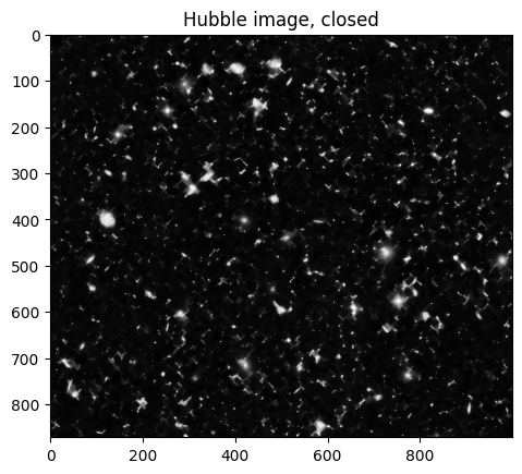
Closing has the effect of first expanding bright objects with the footprint shape (by dilation), followed by trimming those expanded objects (with erosion):
# Recalculate the dilated Hubble image.
hubble_dilated = ski.morphology.dilation(hubble_blue_ubyte, diamond_6)
# Calculate the closing image by eroded the dilated image.
hubble_closed = ski.morphology.erosion(hubble_dilated, diamond_6)
plt.imshow(hubble_closed)
plt.title('Hubble image, closed');
# Is ski.morphology.closing actually the same as erosion on dilation?
np.all(ski.morphology.closing(hubble_blue_ubyte, diamond_6) == hubble_closed)
np.True_
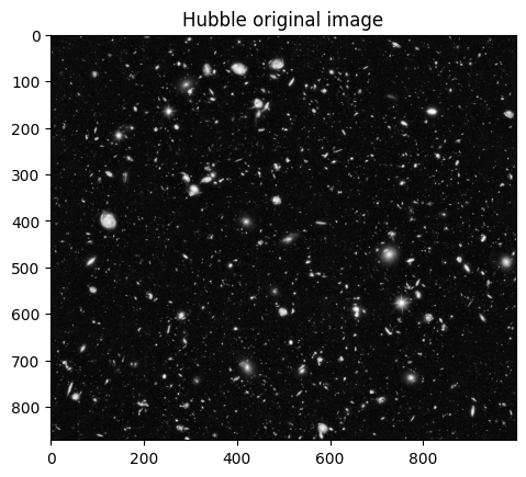
As you can see, in this particular case, the closed image is rather similar to the original, but this will depend, as usual, on the shape and size of the footprint in relation to the objects in the image.
plt.imshow(hubble_blue_ubyte)
plt.title('Hubble original image');
Skeletonizing an image#
In keeping with the horror theme of the xenomorph image, and the legacy of
the smiley array, let’s look at the
ski.morpholoy.skeletonize() function.
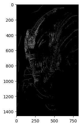
This takes a binary image and finds its “skeleton” - e.g. the centerline of shapes in the image, and marks it out with a single pixel-wide set of lines:
# Skeletonize the xenomorph (skeletonomorph?)
skeletonized_xenomorph = ski.morphology.skeletonize(xenomorph)
plt.imshow(skeletonized_xenomorph);
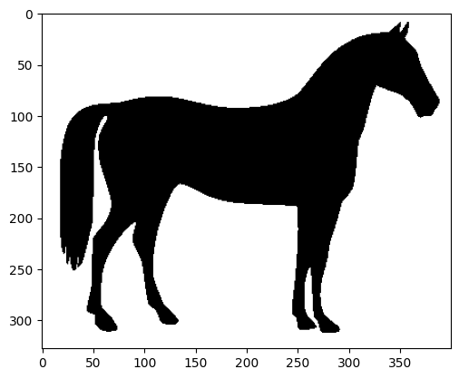
We can also do this with less nightmarish results, to other images, such as the
much more friendly horse from ski.data:
# Import the `horse` image from `ski.data`
horse = ski.data.horse()
plt.imshow(horse);
show_attributes(horse)
Type: <class 'numpy.ndarray'>
dtype: bool
Shape: (328, 400)
Max Pixel Value: True
Min Pixel Value: False
# Skeletonize `horse`.
skeleton_horse = ski.morphology.skeletonize(horse == 0) # The image must be binary numeric, not Boolean, to `skeletonize`.
plt.imshow(skeleton_horse);
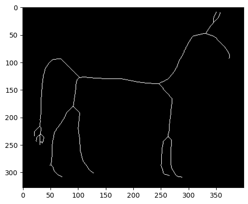
Ok, maybe that is still quite nightmarish…
Summary#
On this page we have looked at fundamental morphological operations in
skimage, and particularly erosion and dilation.
References#
Based on: